Introduction to collocation functions in the quanteda.extras R package

Load the quanteda.extras package

Load the package, as well as others that we’ll use in this vignette.

library(quanteda.extras)
library(quanteda)
library(tidyverse)
library(ggraph)

Prepare the data

First, we’ll use to preprocess_text() function to “clean” the text data. See the preprocess vignette for more information.

sc <- sample_corpus %>%
  mutate(text = preprocess_text(text))

Next, create a corpus and tokenize the data:

sc_tokens <- sc %>%
  corpus() %>% # create a corpus object
  tokens(what="fastestword", remove_numbers=TRUE) # tokenize the data

Collocates by mutual information

The collocates_by_MI() function produces collocation measures (by pointwise mutual information) for a specified token in a quanteda tokens object. In addition to a token, a span or window (as given by a number of words to the left and right of the node word) is required. The default is 5 to the left and 5 to the right.

We’ll start by making a table of tokens that collocate with the token money.

money_collocations <- collocates_by_MI(sc_tokens, "money")

Check the result:

token	col_freq	total_freq	MI_1
10:29	1	1	11.08049
38th	1	1	11.08049
allocations	1	1	11.08049
americanizing	1	1	11.08049
anthedon	1	1	11.08049
assignats	1	1	11.08049

Now, let’s make a similar table for collocates of time.

time_collocations <- collocates_by_MI(sc_tokens, "time")

token	col_freq	total_freq	MI_1
decleat	2	1	10.135473
poignantly	2	1	10.135473
16a	1	1	9.135473
17a	1	1	9.135473
21h	1	1	9.135473
aba	1	1	9.135473

As is clear from the above table, MI is sensitive to rare/infrequent tokens. Because of that sensitivity, it commmon to make thresholds for both token frequency (absolute frequency) and MI score (ususally at some value ≥ 3).

For our purposes, we’ll filter for AF ≥ 5 and MI ≥ 5.

tc <- time_collocations %>% filter(col_freq >= 5 & MI_1 >= 5)
mc <- money_collocations %>% filter(col_freq >= 5 & MI_1 >= 5)

Check the results:

token	col_freq	total_freq	MI_1
warner	6	8	8.720436
cessation	5	7	8.650046
irradiation	5	7	8.650046
lag	5	7	8.650046
wasting	7	11	8.483396
frame	7	16	7.942828

And:

token	col_freq	total_freq	MI_1
owe	5	21	9.010102
raise	10	79	8.098639
extra	6	64	7.665454
spend	10	111	7.608004
insurance	5	64	7.402420
spent	9	122	7.319679

Create a tbl_graph object for plotting

A tbl_graph is a data structure for tidyverse (ggplot2) network plotting.

For this, we’ll use the col_network() function.

net <- col_network(tc, mc)

Plot network

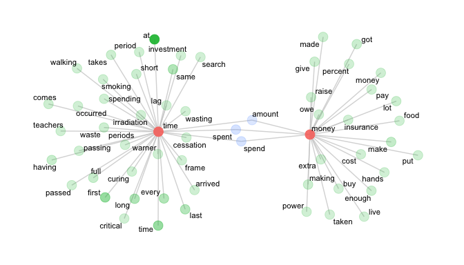
The network plot shows the tokens that distinctly collocate with either time or money, as well as those that interect. The distance from the central tokens (time and money) is governed by the MI score and the transparency (or alpha) is governed by the token frequency.

The aesthetic details of the plot can be manipulated in the various ggraph options.

ggraph(net, weight = link_weight, layout = "stress") + 
  geom_edge_link(color = "gray80", alpha = .75) + 
  geom_node_point(aes(alpha = node_weight, size = 3, color = n_intersects)) +
  geom_node_text(aes(label = label), repel = T, size = 3) +
  scale_alpha(range = c(0.2, 0.9)) +
  theme_graph() +
  theme(legend.position="none")

Bibliography

Brezina, Vaclav. 2018. “Collocation Graphs and Networks: Selected Applications.” In Lexical Collocation Analysis, 59–83. Springer. https://link.springer.com/chapter/10.1007/978-3-319-92582-0_4.

Brezina, Vaclav, Tony McEnery, and Stephen Wattam. 2015. “Collocations in Context: A New Perspective on Collocation Networks.” International Journal of Corpus Linguistics 20 (2): 139–73. https://www.jbe-platform.com/content/journals/10.1075/ijcl.20.2.01bre.

Church, Kenneth, and Patrick Hanks. 1990. “Word Association Norms, Mutual Information, and Lexicography.” Computational Linguistics 16 (1): 22–29. https://aclanthology.org/J90-1003.pdf.