Set 01

The goal of this first lab set is to introduce some fundamental principles of:

• Processing pipelines

• Data presentation and document design

• The affordances and limitations of text data

• The decisions required at every step

Lab 1: Texts, algorithms, and black-boxes

We’re going to start by unpacking the controversy regarding the syuzhet R package. (The readings are short and posted on Canvas.) This is a useful exercise, I think, because it gets to some foundational issues in text analysis – you’re going to encounter them in your work so they’re worth considering from the beginning.

Note

When preparing reports, it is often useful to number your sections. It allows you to point your reader to specific places in your report: See Section 2.1. This is easy to accomplish in Rmarkdown.

Load the cmu.textstat package

Load the package, as well as others that we’ll use in this short lab.

library(cmu.textstat)
library(tidyverse)
library(syuzhet)

The novels that Jockers uses as examples are included as data, which can be accessed as sentiment_data. There are 4 novels, and we’ll check their names stored in the doc_id column.

For this demonstration, we’ll be using Madame Bovary.

doc_id
madame_bovary
portrait_artist
ragged_dick
silas_lapham

Prep the data and calculate sentiment

Next, we do some simple cleaning using str_squish() from the stringr package. Then we’ll split the the novel into sentences and calculate a sentiment score for each.

# str_squish() is a useful function from readr for getting rid of
# extra spaces, carriage returns, etc.
mb <- str_squish(sentiment_data$text[1])

# chunk the novel into sentences
mb_sentences <- get_sentences(mb)

# calculate and return sentiment scores
mb_sentiment <- get_sentiment(mb_sentences)

Let’s check the data:

1.20
0.25
0.00
1.50
1.05
1.20

Transforming the data

The next step is to transform the data. Originally, Jockers used a Fourier transformation, which he described as follows:

Aaron introduced me to a mathematical formula from signal processing called the Fourier transformation. The Fourier transformation provides a way of decomposing a time based signal and reconstituting it in the frequency domain. A complex signal (such as the one seen above in the first figure in this post) can be decomposed into series of symmetrical waves of varying frequencies. And one of the magical things about the Fourier equation is that these decomposed component sine waves can be added back together (summed) in order to reproduce the original wave form–this is called a backward or reverse transformation. Fourier provides a way of transforming the sentiment-based plot trajectories into an equivalent data form that is independent of the length of the trajectory from beginning to end. The frequency domain begins to solve the book length problem.

This introduced some unwanted outcomes, namely that the resulting wave-forms must begin and end at the same point. The updated function uses a Discrete Cosine Transform (DCT), which is commonly used in data compression.

mb_dct <- get_dct_transform(mb_sentiment, low_pass_size = 5, x_reverse_len = 100,
    scale_vals = FALSE, scale_range = TRUE)

mb_dct <- data.frame(dct = mb_dct) %>%
    rownames_to_column("time") %>%
    mutate(time = as.numeric(time))

Check the data:

time	dct
1	1.0000000
2	0.9974733
3	0.9924392
4	0.9849363
5	0.9750217
6	0.9627711

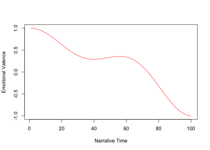
Finally, the values can be plotted.

plot(mb_dct, type = "l", xlab = "Narrative Time", ylab = "Emotional Valence",
    col = "red")

Note

In reports, tables and figures should always be numbered and captioned. As with section numbering, this allows you to refer to tables and figures directly: see Table 2 or Figure 3.1 illustrates…

Transformed vs. non-transformed data

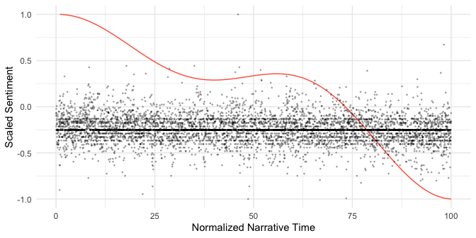
In order to better compare the before vs. after, let’s create a data frame in which we normalize the narrative time values and scale the sentiment scores.

mb_df <- mb_sentiment %>%
    data.frame(sentiment = .) %>%
    rownames_to_column("time") %>%
    mutate(time = as.numeric(time)) %>%
    mutate(time = time/length(mb_sentiment) * 100) %>%
    mutate(sentiment = 2 * (sentiment - min(sentiment))/(max(sentiment) -
        min(sentiment)) - 1)

Now, those values can be plotted with the values extracted from DCT.

ggplot(data = mb_dct, aes(x = time, y = dct)) + geom_line(colour = "tomato") +
    geom_point(data = mb_df, aes(x = time, y = sentiment), alpha = 0.25,
        size = 0.25) + xlab("Normalized Narrative Time") + ylab("Scaled Sentiment") +
    theme_minimal()

What questions does this example raise for you?

This process raises any number of potential questions: about sentiment analysis, about the choice of procedures, about their application to particular kinds of data, to the very choice of the data itself. In asking you to posit your questions, the goal is not to reach any summative conclusion as to whether the syuzhet package is “good” or “bad.” Rather it is to have us think through all of the decisions that we make as analysts (or that get made for us inside R packages, software, etc.), and what we might want to know or test in order to advance and defend our conclusions.

Lab 2: The basics

A simple processing pipeline

Let’s begin by creating an object consisting of a character string. In this case, the first sentence from A Tale of Two Cities.

totc_txt <- "It was the best of times, it was the worst of times, it was the age of wisdom, it was the age of foolishness, it was the epoch of belief, it was the epoch of incredulity, it was the season of Light, it was the season of Darkness, it was the spring of hope, it was the winter of despair."

And we’ll load the tidyverse libraries.

library(tidyverse)

We could then split the vector, say at each space.

totc_tkns <- totc_txt %>%
    str_split(" ")

Then, we can create a table of counts.

totc_df <- table(totc_tkns) %>% # make a table of counts
  as_tibble() %>%
  rename(Token = totc_tkns, AF = n) %>% # rename columns
  arrange(-AF) # sort the data by frequency

Token	AF
of	10
the	10
was	10
it	9
age	2
epoch	2

The process of splitting the string vector into constituent parts is called tokenizing. Think of this as telling the computer how to define a word (or a “token”, which is a more precise, technical term). In this case, we’ve done it in an extremely simple way–by defining a token as any string that is bounded by spaces.

Token	AF
it	9
It	1

Note that in doing so, we are counting capitalized and non-capitalized words as distinct tokens.

There may be specific instances when we want to do this. But normally, we’d want it and It to be the same token. To do that, we can add a step in the processing pipeline that converts our vector to lower case before tokenizing.

totc_df <- tolower(totc_txt) %>%
  str_split(" ") %>%
  table() %>% # make a table of counts
  as_tibble() %>%
  rename(Token = ".", AF = n) %>% # rename columns
  arrange(-AF) # sort the data by frequency

Token	AF
it	10
of	10
the	10
was	10
age	2
epoch	2

What counts as a token?

These choices are important. To carry our any statistical analysis on texts, we radically reorganize texts into counts. Precisely how we choose to do that – the decisions we make in exactly what to count – affects everything else downstream.

For example, you might consider if you want to include numbers? Or symbols? Punctuation? How would you handle hyphenated words? Contractions?

In this short example, how would want your tokenization to handle appreviations like U.S.?

In spite of some problems, we saw a 35% uptick in our user-base in the U.S. But that’s still a lot fewer than we had last year. We’d like to get that number closer to what we’ve experienced in the U.K.–something close to 3 million users.

In one common process, we could convert everything to lowercase and remove puctuation. We would, then, end up with the token us. Is that acceptable, given the data and analytical task?

That said, we also need to bear in mind that as analysts, we are often building models, creating representations, or testing hypotheses. Under most conditions, there will always be error introduced through the collection and preparation of our text data.

The point (generally) is not to perfectly mimic what our human brain understands to be a “word.” It is to make decisions that best serve our analytical task and to be able to articulate our reasons for those decisions. Sometimes, that might even mean tokenizing in a way that takes advange of computational power, but is decidely more difficult for a human reader to parse.

Lab 3: Processing piplines

Tokenizing with quanteda

In the previous lab, we did some back-of-the-napkin text processing. In that lab, you were encouraged to think about what exactly is happening when you split a text into tokens and convert those into counts.

We’ll build on that foundational work, but let an R package quanteda do some of the heavy lifting for us. So let’s load our packages:

library(cmu.textstat)
library(tidyverse)
library(quanteda)
library(quanteda.textstats)

And again, we’ll start with the first sentence from A Tale of Two Cities.

totc_txt <- "It was the best of times, it was the worst of times, it was the age of wisdom, it was the age of foolishness, it was the epoch of belief, it was the epoch of incredulity, it was the season of Light, it was the season of Darkness, it was the spring of hope, it was the winter of despair."

Create a corpus

The first step is to create a corpus object:

totc_corpus <- corpus(totc_txt)

And see what we have:

Text	Types	Tokens	Sentences
text1	23	70	1

Note that if we had more than 1 document, we would get a count of how many documents in which the token appear, and that we can assign documents to grouping variable. This will become useful later.

Tokenize the corpus

totc_tkns <- tokens(totc_corpus, what = "word", remove_punct = TRUE)

Create a document-feature matrix (dfm)

totc_dfm <- dfm(totc_tkns)

A dfm is an important data structure to understand, as it often serves as the foundation for all kinds of downstream statistical processing. It is a table with rows for documents (or observations) and columns for tokens (or variables)

doc_id	it	was	the	best	of	times	worst	age	wisdom	foolishness	epoch
text1	10	10	10	1	10	2	1	2	1	1	2

And count our tokens

This is done using the textstat_frequency() function from quanteda.textstats: textstat_frequency(totc_dfm)

feature	frequency	rank	docfreq	group
it	10	1	1	all
was	10	1	1	all
the	10	1	1	all
of	10	1	1	all
times	2	5	1	all
age	2	5	1	all
epoch	2	5	1	all
season	2	5	1	all
best	1	9	1	all
worst	1	9	1	all
wisdom	1	9	1	all
foolishness	1	9	1	all
belief	1	9	1	all
incredulity	1	9	1	all
light	1	9	1	all
darkness	1	9	1	all
spring	1	9	1	all
hope	1	9	1	all
winter	1	9	1	all
despair	1	9	1	all

Using pipes to expidite the process

This time, we will change remove_punct to FALSE.

totc_freq <- totc_corpus %>%
    tokens(what = "word", remove_punct = FALSE) %>%
    dfm() %>%
    textstat_frequency()

feature	frequency	rank	docfreq	group
it	10	1	1	all
was	10	1	1	all
the	10	1	1	all
of	10	1	1	all
,	9	5	1	all
times	2	6	1	all
age	2	6	1	all
epoch	2	6	1	all
season	2	6	1	all
best	1	10	1	all
worst	1	10	1	all
wisdom	1	10	1	all
foolishness	1	10	1	all
belief	1	10	1	all
incredulity	1	10	1	all
light	1	10	1	all
darkness	1	10	1	all
spring	1	10	1	all
hope	1	10	1	all
winter	1	10	1	all
despair	1	10	1	all
.	1	10	1	all

Tokenizing options

In the previous lab, you were asked to consider the questions: What counts as a token/word? And how do you tell the computer to count what you want?

As the above code block suggest, the tokens() function in quanteda gives you some measure on control.

We’ll read in a more complex string:

text_2 <- "Jane Austen was not credited as the author of 'Pride and Prejudice.' In 1813, the title page simply read \"by the author of Sense and Sensibility.\" It wasn't until after Austen's death that her identity was revealed. #MentalFlossBookClub with @HowLifeUnfolds #15Pages https://pbs.twimg.com/media/EBOUqbfWwAABEoj.jpg"

And process it as we did earlier.

text_2_freq <- text_2 %>%
    corpus() %>%
    tokens(what = "word", remove_punct = TRUE) %>%
    dfm() %>%
    textstat_frequency()

feature	frequency	rank	docfreq	group
the	3	1	1	all
was	2	2	1	all
author	2	2	1	all
of	2	2	1	all
and	2	2	1	all
jane	1	6	1	all
austen	1	6	1	all
not	1	6	1	all
credited	1	6	1	all
as	1	6	1	all
pride	1	6	1	all
prejudice	1	6	1	all
in	1	6	1	all
1813	1	6	1	all
title	1	6	1	all
page	1	6	1	all
simply	1	6	1	all
read	1	6	1	all
by	1	6	1	all
sense	1	6	1	all
sensibility	1	6	1	all
it	1	6	1	all
wasn’t	1	6	1	all
until	1	6	1	all
after	1	6	1	all
austen’s	1	6	1	all
death	1	6	1	all
that	1	6	1	all
her	1	6	1	all
identity	1	6	1	all
revealed	1	6	1	all
#mentalflossbookclub	1	6	1	all
with	1	6	1	all
@howlifeunfolds	1	6	1	all
#15pages	1	6	1	all
https://pbs.twimg.com/media/ebouqbfwwaabeoj.jpg	1	6	1	all

Note that in addition to various logical “remove” arguments (remove_punct, remove_symbols, etc.), the tokens() function has a what argument. The default, “word”, is “smarter”, but also slower. Another option is “fastestword”, which splits at spaces.

text_2_freq <- text_2 %>%
    corpus() %>%
    tokens(what = "fastestword", remove_punct = TRUE, remove_url = TRUE) %>%
    dfm() %>%
    textstat_frequency() %>%
    as_tibble() %>%
    dplyr::select(feature, frequency)

feature	frequency
the	3
was	2
author	2
of	2
and	2
jane	1
austen	1
not	1
credited	1
as	1
’pride	1
prejudice.’	1
in	1
1813,	1
title	1
page	1
simply	1
read	1
“by	1
sense	1
sensibility.”	1
it	1
wasn’t	1
until	1
after	1
austen’s	1
death	1
that	1
her	1
identity	1
revealed.	1
#mentalflossbookclub	1
with	1
@howlifeunfolds	1
#15pages	1

This, of course, makes no difference with just a few tokens, but does if you’re trying to process millions.

Also note that we’ve used the select() function to choose specific columns.

Pre-processing

An alternative to making tokenizing decisions inside the tokenizing process, you can process the text before tokenizing using functions for manipulating strings in stringr, stringi, textclean, or base R (like grep()). Some common and convenient transformations are wrapped in a cmu.textstat function called preprocess_text()

text_2_freq <- text_2 %>%
  preprocess_text() %>%
  corpus() %>%
  tokens(what = "fastestword") %>%
  dfm() %>%
  textstat_frequency() %>%
  as_tibble() %>%
  dplyr::select(feature, frequency) %>%
  rename(Token = feature, AF = frequency) %>% # for absolute frequency
  mutate(New = NA)

Token	AF	New
was	3	NA
the	3	NA
austen	2	NA
author	2	NA
of	2	NA
and	2	NA
jane	1	NA
not	1	NA
credited	1	NA
as	1	NA
pride	1	NA
prejudice	1	NA
in	1	NA
1813	1	NA
title	1	NA
page	1	NA
simply	1	NA
read	1	NA
by	1	NA
sense	1	NA
sensibility	1	NA
it	1	NA
n’t	1	NA
until	1	NA
after	1	NA
s	1	NA
death	1	NA
that	1	NA
her	1	NA
identity	1	NA
revealed	1	NA
mentalflossbookclub	1	NA
with	1	NA
howlifeunfolds	1	NA
15pages	1	NA
pbs.twimg.com/media/ebouqbfwwaabeoj.jpg	1	NA

Note how the default arguments treat negation and possessive markers. As with the tokens () function, many of these options are logical.

Note, too, that we’ve renamed the columns and added a new one using mutate().

Creating a corpus composition table

Whenever you report the results of a corpus-based analysis, it is best practice to include a table that summarizes the composition of your corpus (or corpora) and any relevant variables. Most often this would include token counts aggregated by relevant categorical variables and a row of totals.

Here is an example from Hyland & Jiang (2016):

Adding a grouping variable

We have 2 short texts (one from fiction and one from Twitter). Let’s first combine them into a single corpus. First, a data frame is created that has 2 columns (doc_id and text). Then, the text column is passed to the preprocess_text() function before creating the corpus.

comb_corpus <- data.frame(doc_id = c("text_1", "text_2"), text = c(totc_txt,
    text_2)) %>%
    mutate(text = preprocess_text(text)) %>%
    corpus()

Next well assign a grouping variable using docvars(). In later labs, we’ll use a similar process to assign variables from tables of metadata.

Note

This works in much the same way as assigning addributes.

docvars(comb_corpus) <- data.frame(text_type = c("Fiction", "Twitter"))

Now we can tokenize.

comb_tkns <- comb_corpus %>%
    tokens(what = "fastestword")

Once we have done this, we can use that grouping variable to manipulate the data in a vraiety of ways. We could use dfm_group() to aggregate by group instead of individual text. (Though because we have only 2 texts here, it amounts to the same thing.)

comb_dfm <- dfm(comb_tkns) %>%
    dfm_group(groups = text_type)

doc_id	it	was	the	best	of	times	worst	age	wisdom	foolishness
Fiction	10	10	10	1	10	2	1	2	1	1
Twitter	1	3	3	0	2	0	0	0	0	0

Or we can return a frequency table with a group column.

comb_freq <- dfm(comb_tkns) %>%
    textstat_frequency(groups = text_type)

feature	frequency	rank	docfreq	group
it	10	1	1	Fiction
was	10	1	1	Fiction
the	10	1	1	Fiction
of	10	1	1	Fiction
was	3	1	1	Twitter
the	3	1	1	Twitter
of	2	3	1	Twitter
austen	2	3	1	Twitter
author	2	3	1	Twitter
and	2	3	1	Twitter

An additional option would be to use the ntoken() function to collect the total counts by text and combine those in a data frame with the docvars():

comb_ntoken <- data.frame("Tokens" = ntoken(comb_tkns), docvars(comb_tkns))

-	Tokens	text_type
text_1	60	Fiction
text_2	44	Twitter

Note

With either the comb_freq or the comb_ntoken structures above, creating a corpus composition table would require summing counts by the categorical variable text_type. (In this simple example, of course, we would not need to so with comb_ntoken, since we only have 2 texts.)

There are a variety of ways of generating sums by categorical variables. One easy way is to use group_by and summarize().

Similarly, adding a Total row is simple with adorn_totals() from janitor.

The composition table in this toy example would produce something like this:

Text Type	Tokens
Fiction	60
Twitter	44
Total	104