Set 03

Lab 7: Part-of-speech tagging and dependency parsing

In the previous lab, we worked with keyness and effect sizes, specifically using log-likelihood and log ratio measures.

We are now going to add to our toolkit by using the same measures, but applied to data that has been tagged and parsed. To our processing pipeline, we will be adding udpipe.

What does udpipe do?

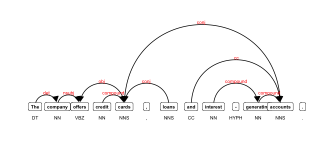
Before we start processing in R, let’s get some sense of what “universal dependency parsing” is and what its output looks like.

Parse a sample sentence online

Go to this webpage: http://lindat.mff.cuni.cz/services/udpipe/.

And paste the following sentence into the text field:

The company offers credit cards, loans and interest-generating accounts.

Set the model to english-ewt-ud. Then, click the “Process Input” button. You should now see an output. If you choose the “Table” tab, you can view the output in a tablular format:

Id	Form	Lemma	UPosTag	XPosTag	Feats	Head	DepRel	Deps	Misc
1	The	the	DET	DT	Definite=Def|PronType=Art	2	det	_	TokenRange=0:3
2	company	company	NOUN	NN	Number=Sing	3	nsubj	_	TokenRange=4:11
3	offers	offer	VERB	VBZ	Mood=Ind|Number=Sing|Person=3|Tense=Pres|VerbForm=Fin	0	root	_	TokenRange=12:18
4	credit	credit	NOUN	NN	Number=Sing	5	compound	_	TokenRange=19:25
5	cards	card	NOUN	NNS	Number=Plur	3	obj	_	SpaceAfter=No|TokenRange=26:31
6	,	,	PUNCT	,	_	7	punct	_	TokenRange=31:32
7	loans	loan	NOUN	NNS	Number=Plur	5	conj	_	TokenRange=33:38
8	and	and	CCONJ	CC	_	12	cc	_	TokenRange=39:42
9	interest	interest	NOUN	NN	Number=Sing	11	compound	_	SpaceAfter=No|TokenRange=43:51
10	-	-	PUNCT	HYPH	_	11	punct	_	SpaceAfter=No|TokenRange=51:52
11	generating	generate	NOUN	NN	Number=Sing	12	compound	_	TokenRange=52:62
12	accounts	account	NOUN	NNS	Number=Plur	5	conj	_	SpaceAfter=No|TokenRange=63:71
13	.	.	PUNCT	.	_	3	punct	_	SpaceAfter=No|TokenRange=71:72

Basic parse structure

There is a column for the token and one for the token’s base form or lemma.

Those are followed by a tag for the general lexical class or “universal part-of-speech” (upos) tag, and a tree-bank specific (xpos) part-of-speech tag.

The xpos tags are Penn Treebank tags.

The part-of-speech tags are followed by a column of integers that refer to the id of the token that is at the head of the dependency structure, which is followed by the dependency relation identifier.

Visualize the dependency

From the “Output Text” tab, copy the output start with the sent_id including the pound sign

Paste the information into the text field here: https://urd2.let.rug.nl/~kleiweg/conllu/.

Then click the “Submit Query” button below the text field. This should generate a visualization of the dependency structure.

Load the needed packages

library(cmu.textstat)
library(tidyverse)
library(quanteda)
library(quanteda.textstats)
library(udpipe)

Parsing

Preparing a corpus

When we parse texts using a model like ones available in udpipe or spacy, we need to do very little to prepare the corpus. We could trim extra spaces and returns using str_squish() or remove urls, but generally we want the text to be mostly “as is” so the model can do its job.

Download a model

You only need to run this line of code once. To run it, remove the pound sign, run the line, then add the pound sign after you’ve downloaded the model. Or you can run the next chunk and the model will automatically be downloaded in your working directory.

# udpipe_download_model(language = "english")

Annotate a sentence

txt <- "The company offers credit cards, loans and interest-generating accounts."
annotation <- udpipe(txt, "english")

doc_id	paragraph_id	sentence_id	sentence	start	end	term_id	token_id	token	lemma	upos	xpos	feats	head_token_id	dep_rel	deps	misc
doc1	1	1	The company offers credit cards, loans and interest-generating accounts.	1	3	1	1	The	the	DET	DT	Definite=Def|PronType=Art	2	det	NA	NA
doc1	1	1	The company offers credit cards, loans and interest-generating accounts.	5	11	2	2	company	company	NOUN	NN	Number=Sing	3	nsubj	NA	NA
doc1	1	1	The company offers credit cards, loans and interest-generating accounts.	13	18	3	3	offers	offer	VERB	VBZ	Mood=Ind|Number=Sing|Person=3|Tense=Pres|VerbForm=Fin	0	root	NA	NA
doc1	1	1	The company offers credit cards, loans and interest-generating accounts.	20	25	4	4	credit	credit	NOUN	NN	Number=Sing	5	compound	NA	NA
doc1	1	1	The company offers credit cards, loans and interest-generating accounts.	27	31	5	5	cards	card	NOUN	NNS	Number=Plur	3	obj	NA	SpaceAfter=No
doc1	1	1	The company offers credit cards, loans and interest-generating accounts.	32	32	6	6	,	,	PUNCT	,	NA	7	punct	NA	NA
doc1	1	1	The company offers credit cards, loans and interest-generating accounts.	34	38	7	7	loans	loans	NOUN	NNS	Number=Plur	5	conj	NA	NA
doc1	1	1	The company offers credit cards, loans and interest-generating accounts.	40	42	8	8	and	and	CCONJ	CC	NA	12	cc	NA	NA
doc1	1	1	The company offers credit cards, loans and interest-generating accounts.	44	51	9	9	interest	interest	NOUN	NN	Number=Sing	11	compound	NA	SpaceAfter=No
doc1	1	1	The company offers credit cards, loans and interest-generating accounts.	52	52	10	10	-	-	PUNCT	HYPH	NA	11	punct	NA	SpaceAfter=No
doc1	1	1	The company offers credit cards, loans and interest-generating accounts.	53	62	11	11	generating	genera	NOUN	NN	Number=Sing	12	compound	NA	NA
doc1	1	1	The company offers credit cards, loans and interest-generating accounts.	64	71	12	12	accounts	account	NOUN	NNS	Number=Plur	5	conj	NA	SpaceAfter=No
doc1	1	1	The company offers credit cards, loans and interest-generating accounts.	72	72	13	13	.	.	PUNCT	.	NA	3	punct	NA	SpacesAfter=No

Plot the annotation

We can also plot the dependency structure using igraph:

library(igraph)
library(ggraph)

First we’ll create a plotting function.

plot_annotation <- function(x, size = 3){
  stopifnot(is.data.frame(x) & all(c("sentence_id", "token_id", "head_token_id", "dep_rel",
                                     "token_id", "token", "lemma", "upos", "xpos", "feats") %in% colnames(x)))
  x <- x[!is.na(x$head_token_id), ]
  x <- x[x$sentence_id %in% min(x$sentence_id), ]
  edges <- x[x$head_token_id != 0, c("token_id", "head_token_id", "dep_rel")]
  edges <- edges[edges$dep_rel != "punct",]
  edges$head_token_id <- ifelse(edges$head_token_id == 0, edges$token_id, edges$head_token_id)
  nodes = x[, c("token_id", "token", "lemma", "upos", "xpos", "feats")]
  edges$label <- edges$dep_rel
  g <- graph_from_data_frame(edges,
                             vertices = nodes,
                             directed = TRUE)
  ggraph(g, layout = "linear") +
    geom_edge_arc(ggplot2::aes(label = dep_rel, vjust = -0.20), fold = T,linemitre = 2,
                  arrow = grid::arrow(length = unit(3, 'mm'), ends = "last", type = "closed"),
                  end_cap = ggraph::label_rect("wordswordswords"),
                  label_colour = "red", check_overlap = TRUE, label_size = size) +
    geom_node_label(ggplot2::aes(label = token), col = "black", size = size, fontface = "bold") +
    geom_node_text(ggplot2::aes(label = xpos), nudge_y = -0.35, size = size) +
    theme_graph(base_family = "Arial Narrow")
}

And plot the annotation:

plot_annotation(annotation, size = 2.5)

Annotate a corpus

Parsing text is a computationally intensive process and can take time. So for the purposes of this lab, we’ll create a smaller sub-sample of the the data. By adding a column called text_type which includes information extracted from the file names, we can sample 5 texts from each.

set.seed(123)
sub_corpus <- quanteda.extras::sample_corpus %>%
  mutate(text_type = str_extract(doc_id, "^[a-z]+")) %>%
  group_by(text_type) %>%
  sample_n(5) %>%
  ungroup() %>%
  dplyr::select(doc_id, text)

Parallel processing

Parallel processing is a method whereby separate parts of an overall complex task are broken up and run simultaneously on multiple CPUs, thereby reducing the amount of time for processing. Part-of-speech tagging and dependency parsing are computationally intensive, so using parallel processing can save valuable time.

The udpipe() function has an argument for assigning cores: parallel.cores = 1L. It’s easy to set up, so feel free to use that option.

A second option, requires more preparation, but is even faster. So we’ll walk through how it works. First, we will split the corpus based on available cores.

corpus_split <- split(sub_corpus, seq(1, nrow(sub_corpus), by = 10))

For parallel processing in R, we’ll us the package future.apply.

library(future.apply)

Next, we set up our parallel session by specifying the number of cores, and creating a simple annotation function.

ncores <- 4L
plan(multisession, workers = ncores)

annotate_splits <- function(corpus_text) {
  ud_model <- udpipe_load_model("english-ewt-ud-2.5-191206.udpipe")
  x <- data.table::as.data.table(udpipe_annotate(ud_model, x = corpus_text$text,
                                                 doc_id = corpus_text$doc_id))
  return(x)
}

Finally, we annotate using future_lapply. On my machine, this takes roughly 32 seconds.

annotation <- future_lapply(corpus_split, annotate_splits, future.seed = T)

As you might guess, the output is a list of data frames, so we’ll combine them using rbindlist().

annotation <- data.table::rbindlist(annotation)

Process with quanteda

Format the data for quanteda

If we want to do any further processing in quanteda, we need to make a couple of adjustments to our data frame.

anno_edit <- annotation %>%
  dplyr::select(doc_id, sentence_id, token_id, token, lemma, upos, xpos, head_token_id, dep_rel) %>%
  rename(pos = upos, tag = xpos)

anno_edit <- structure(anno_edit, class = c("spacyr_parsed", "data.frame"))

Convert to tokens

sub_tkns <- as.tokens(anno_edit, include_pos = "tag", concatenator = "_")

Create a dfm

We will also extract and assign the variable text_type to the tokens object.

doc_categories <- names(sub_tkns) %>%
  data.frame(text_type = .) %>%
  mutate(text_type = str_extract(text_type, "^[a-z]+"))

docvars(sub_tkns) <- doc_categories

sub_dfm <- dfm(sub_tkns)

And check the frequencies:

feature	frequency	rank	docfreq	group	end	term_id	token_id	token	lemma	upos	xpos	feats	head_token_id	dep_rel	deps	misc
._.	6452	1	40	all	3	1	1	The	the	DET	DT	Definite=Def|PronType=Art	2	det	NA	NA
,_,	5900	2	40	all	11	2	2	company	company	NOUN	NN	Number=Sing	3	nsubj	NA	NA
the_dt	5217	3	40	all	18	3	3	offers	offer	VERB	VBZ	Mood=Ind|Number=Sing|Person=3|Tense=Pres|VerbForm=Fin	0	root	NA	NA
and_cc	2596	4	40	all	25	4	4	credit	credit	NOUN	NN	Number=Sing	5	compound	NA	NA
of_in	2513	5	40	all	31	5	5	cards	card	NOUN	NNS	Number=Plur	3	obj	NA	SpaceAfter=No
a_dt	2256	6	40	all	32	6	6	,	,	PUNCT	,	NA	7	punct	NA	NA
to_to	1702	7	40	all	38	7	7	loans	loans	NOUN	NNS	Number=Plur	5	conj	NA	NA
in_in	1645	8	40	all	42	8	8	and	and	CCONJ	CC	NA	12	cc	NA	NA
i_prp	1497	9	36	all	51	9	9	interest	interest	NOUN	NN	Number=Sing	11	compound	NA	SpaceAfter=No
you_prp	1202	10	36	all	52	10	10	-	-	PUNCT	HYPH	NA	11	punct	NA	SpaceAfter=No

Filter/select tokens

Warning

There are multiple ways to filter/select the tokens we want to count. We could, for example, just filter out all rows in the annotation data frame tagged as PUNCT, if we wanted to exclude punctuation from our counts.

I would, however, advise against altering the original parsed file. We may want to try different options, and we want to avoid having to re-parse our corpus, as that is the most computationally intensive step in the processing pipeline. In fact, if this were part of an actual project, I would advise that you save the parsed data frame as a .csv file using write_csv() or as an .rda file for later use.

We will use the tokens_select() function to either keep or remove tokens based on regular expressions.

sub_dfm <- sub_tkns %>%
  tokens_select("^.*[a-zA-Z0-9]+.*_[a-z]", selection = "keep", valuetype = "regex", case_insensitive = T) %>%
  dfm()

And check the frequencies:

feature	frequency	rank	docfreq	group	end	term_id	token_id	token	lemma	upos	xpos	feats	head_token_id	dep_rel	deps	misc
the_dt	5217	1	40	all	3	1	1	The	the	DET	DT	Definite=Def|PronType=Art	2	det	NA	NA
and_cc	2596	2	40	all	11	2	2	company	company	NOUN	NN	Number=Sing	3	nsubj	NA	NA
of_in	2513	3	40	all	18	3	3	offers	offer	VERB	VBZ	Mood=Ind|Number=Sing|Person=3|Tense=Pres|VerbForm=Fin	0	root	NA	NA
a_dt	2256	4	40	all	25	4	4	credit	credit	NOUN	NN	Number=Sing	5	compound	NA	NA
to_to	1702	5	40	all	31	5	5	cards	card	NOUN	NNS	Number=Plur	3	obj	NA	SpaceAfter=No
in_in	1645	6	40	all	32	6	6	,	,	PUNCT	,	NA	7	punct	NA	NA
i_prp	1497	7	36	all	38	7	7	loans	loans	NOUN	NNS	Number=Plur	5	conj	NA	NA
you_prp	1202	8	36	all	42	8	8	and	and	CCONJ	CC	NA	12	cc	NA	NA
it_prp	1168	9	39	all	51	9	9	interest	interest	NOUN	NN	Number=Sing	11	compound	NA	SpaceAfter=No
is_vbz	1042	10	40	all	52	10	10	-	-	PUNCT	HYPH	NA	11	punct	NA	SpaceAfter=No

If we want to compare one text-type (as our target corpus) to another (as our reference corpus), we can easily subset the data.

acad_dfm <- dfm_subset(sub_dfm, text_type == "acad") %>% dfm_trim(min_termfreq = 1)
fic_dfm <- dfm_subset(sub_dfm, text_type == "fic") %>% dfm_trim(min_termfreq = 1)

And finally, we can generate a keyness table,

acad_v_fic <- keyness_table(acad_dfm, fic_dfm) %>%
  separate(col = Token, into = c("Token", "Tag"), sep = "_")

Token	Tag	LL	LR	PV	AF_Tar	AF_Ref	Per_10.4_Tar	Per_10.4_Ref	DP_Tar	DP_Ref
of	in	254.97151	1.8779434	0	563	159	445.02411	121.078282	0.0937508	0.0673735
japan	nnp	69.77395	6.6685451	0	49	0	38.73212	0.000000	0.7559586	NA
methylation	nn	68.34999	6.6387977	0	48	0	37.94166	0.000000	0.8039681	NA
smoking	nn	66.92604	6.6084241	0	47	0	37.15121	0.000000	0.7826915	NA
china	nnp	58.38229	6.4113872	0	41	0	32.40851	0.000000	0.5975812	NA
japanese	jj	48.41458	6.1412981	0	34	0	26.87535	0.000000	0.7967750	NA
the	dt	40.62914	0.4889023	0	822	608	649.75101	462.991167	0.1385967	0.1397936
by	in	38.86344	1.7319071	0	96	30	75.88333	22.844959	0.1877124	0.1651132
chinese	jj	37.02291	5.7542749	0	26	0	20.55174	0.000000	0.5975812	NA
sauropods	nns	34.17500	5.6387977	0	24	0	18.97083	0.000000	0.7980397	NA
intensity	nn	32.75104	5.5773972	0	23	0	18.18038	0.000000	0.7604898	NA
united	nnp	32.75104	5.5773972	0	23	0	18.18038	0.000000	0.5971860	NA
these	dt	31.63882	3.5563356	0	34	3	26.87535	2.284496	0.3953349	0.6019647
states	nnp	31.32708	5.5132668	0	22	0	17.38993	0.000000	0.5971860	NA
as	in	30.26069	1.4791411	0	94	35	74.30243	26.652452	0.0836651	0.4012032

From that data, we can filter specific lexical classes, like modal verbs:

Token	Tag	LL	LR	PV	AF_Tar	AF_Ref	Per_10.4_Tar	Per_10.4_Ref	DP_Tar	DP_Ref
may	md	3.9877692	1.4323469	0.0458317	13	5	10.2758675	3.8074931	0.1648517	0.4012032
will	md	3.6584302	1.1412981	0.0557862	17	8	13.4376729	6.0919890	0.5387577	0.5992994
ill	md	1.4239582	1.0538352	0.2327530	1	0	0.7904513	0.0000000	0.7967750	NA
ought	md	1.4239582	1.0538352	0.2327530	1	0	0.7904513	0.0000000	0.8004110	NA
must	md	0.1321795	0.3168696	0.7161829	6	5	4.7427081	3.8074931	0.4305193	0.6019647
wo	md	0.0006962	0.0538352	0.9789499	1	1	0.7904513	0.7614986	0.7967750	0.7996497
ca	md	-0.1657799	-0.5311273	0.6838899	2	3	1.5809027	2.2844959	0.7967750	0.5992994
should	md	-0.2169360	-0.3612023	0.6413845	6	8	4.7427081	6.0919890	0.2614813	0.3464819
can	md	-3.3401792	-0.8041458	0.0676072	16	29	12.6472216	22.0834602	0.3475812	0.2237178
might	md	-3.6344817	-1.9461648	0.0565942	2	8	1.5809027	6.0919890	0.5984507	0.6765535
could	md	-6.1468621	-0.9129979	0.0131645	22	43	17.3899296	32.7444411	0.2592573	0.2407274
would	md	-9.2158449	-1.3087349	0.0023993	14	36	11.0663189	27.4139507	0.3131317	0.2149795
’ll	md	-12.9666315	-3.7535197	0.0003171	1	14	0.7904513	10.6609808	0.7967750	0.2393390
’d	md	-32.3838413	-5.5311273	0.0000000	0	24	0.0000000	18.2759671	NA	0.2340339

Extract phrases

We can also extract phrases of specific types. To so so, we first use the function as_phrasemachine() to add a new column to our annotation called phrase_tag.

annotation$phrase_tag <- as_phrasemachine(annotation$upos, type = "upos")

Next, we can use the function keywords_phrases() to extract phrase-types based on regular expressions. Refer to the documentation for suggested regex patterns.

You can also read examples of use cases.

First, we’ll subset our data into annotations by text-type.

acad_anno <- annotation %>% filter(str_detect(doc_id, "acad"))
fic_anno <- annotation %>% filter(str_detect(doc_id, "fic"))

acad_nps <- keywords_phrases(x = acad_anno$phrase_tag, term = tolower(acad_anno$token), 
                          pattern = "(A|N)*N(P+D*(A|N)*N)*", 
                          is_regex = TRUE, detailed = T)


fic_nps <- keywords_phrases(x = fic_anno$phrase_tag, term = tolower(fic_anno$token), 
                             pattern = "(A|N)*N(P+D*(A|N)*N)*", 
                             is_regex = TRUE, detailed = T)

keyword	ngram	pattern	start	end
largest creatures	2	AN	2	3
creatures	1	N	3	3
earth	1	N	9	9
animals	1	N	11	11
apatosaurus	1	N	14	14
aka	1	N	16	16
aka brontosaurus	2	NN	16	17
brontosaurus	1	N	17	17
paleontologists	1	N	19	19
picture	1	N	23	23
they	1	N	26	26
english anatomist	2	AN	35	36
anatomist	1	N	36	36
paleontologist	1	N	39	39
paleontologist richard	2	NN	39	40

Note that although the function uses the term keywords, it is NOT executing a hypothesis test of any kind.

Extract only unique phrases

Note that udpipe extracts overlapping constituents of phrase structures. Normally, we would want only unique phrases. To find those we’ll take advantage of the start and end indexes, using the between() function from the data.table package.

That will generate a logical vector, which we can use to filter out only those phrases that don’t overlap with another.

idx <- seq(1:nrow(acad_nps))

is_unique <- lapply(idx, function(i) sum(data.table::between(acad_nps$start[i], acad_nps$start, acad_nps$end) & data.table::between(acad_nps$end[i], acad_nps$start, acad_nps$end)) == 1) %>% unlist()

acad_nps <- acad_nps[is_unique, ]

idx <- seq(1:nrow(fic_nps))

is_unique <- lapply(idx, function(i) sum(data.table::between(fic_nps$start[i], fic_nps$start, fic_nps$end) & data.table::between(fic_nps$end[i], fic_nps$start, fic_nps$end)) == 1) %>% unlist()

fic_nps <- fic_nps[is_unique, ]

We can also add a rough accounting of the lengths of the noun phrases by summing the spaces and adding 1.

acad_nps <- acad_nps %>%
  mutate(phrase_length = str_count(keyword, " ") + 1)

fic_nps <- fic_nps %>%
  mutate(phrase_length = str_count(keyword, " ") + 1)

keyword	ngram	pattern	start	end	phrase_length
it	1	N	1	1	1
pleasant summer night	3	ANN	4	6	3
wind off the ocean	4	NPDN	10	13	4
trees along copley square	4	NPNN	16	19	4
i	1	N	21	21	1
boston public library	3	NNN	25	27	3
square	1	N	31	31	1
copley plaza bar	3	NNN	37	39	3
first time	2	AN	44	45	2
sammy	1	N	47	47	1
piano	1	N	50	50	1
his music	2	NN	53	54	2
talk of the crowd	4	NPDN	58	61	4
sammy	1	N	64	64	1
ease	1	N	68	68	1

Lab 8: Logistic Regression

This is a script that walks you through basic logistic and multinomial regression. Logistic regression can be applied to binary variables. In our textbook, Brezina walks though an examples applied to lexico-grammar. What are the conditions that predict whether the definite article (“the”) or the indefinite article (“a”) occur? Or predict which relative pronoun (“that” or “which”) is used?

Multinomial regression can be applied to situations where we have more than 2 outcome variables AND those categories are UNORDERED. Here, we’ll look at writing in the Humanities, Sciences, and Social Sciences. There is not inherent order to these categories. If we did have ORDERED categories, we would use ordinal regression. These are very similar procedures, with similar reporting conventions.

We’re going to start by preparing a versions of the that/which data that Brezina describes starting on pg. 130

We have student writing from the US in the MICUSP data and from the UK in the BAWE data. Rather than going through the tagging process, we’ll load in some data that’s already been tagged using udpipe and the Penn-Treebank tagset

https://www.ling.upenn.edu/courses/Fall_2003/ling001/penn_treebank_pos.html

Load the needed packages

library(cmu.textstat)
library(tidyverse)
library(quanteda)
library(nnet)

Case 1

Preparing linguistic data for logistic regression is often a complex process, as it will be for this lab. Our problem comes from Brezina (pg. 130) and concerns that vs. which:

While writing this chapter, I encountered the following situation: my word processor underlines with a wiggly line a phrse that included the relative pronoun which, signaling a potential grammatical error or inaccuracy. The correction off correction offered was to either add a comma in front of which or use the relative pronoun that instead, with the reasoning being as follows: ‘If these words are not essential to the meaning of your sentences, use “which” and separate the words with a comma.’

We are going to mimic Brezina’s experiment, but instead of using the BE06 and AmE06 corpora, we will use the Michigan Corpus of Upper-Level Student Papers (MICUSP) and the British Academic Written English corpus (BAWE).

To save time, the data has already been tagged with udpipe using the follow code.

udmodel <- udpipe_load_model(file = "english-ewt-ud-2.5-191206.udpipe")
target_folder <- "/Users/user/Downloads/bawe_udpipe/"
files_list <- list.files("/Users/user/Downloads/bawe_body", full.names = T)

tag_text <- function(x){
  
  file_name <- basename(x) %>% str_remove(".txt")
  output_file <- paste0(target_folder, file_name, "_udp.txt")
  txt <- readr::read_file(x) %>% str_squish()
  annotation <- udpipe_annotate(udmodel, txt, parser = "none") %>% 
    as.data.frame() %>%
    dplyr::select(token, xpos) %>%
    unite("token", token:xpos)
  
  new_txt <- paste(annotation$token, collapse=" ")
  write.table(new_txt, output_file, quote = F, row.names = F, col.names = F)
  
}

lapply(files_list, tag_text)

Note

In this case, tags are being embedded. That is, the token is being linked to the tag with an underscore: Throughout_IN history_NN. However, the same principle of tagging a text (or a subset of texts) then writing out the result to a local file is one way to handle the computational demands of parsing. For example, you could take the vector of file paths, split it into chunks of say 10, then iterate along those chunks, writing out each result as it progresses. That way, you eliminate the need to put everything into memory at the same time. After the files have been created, they can be joined for analysis.

Prepare tokens

Download and unzip the data from Canvas.

us_files_list <- list.files("/Users/user/Downloads/micusp_udpipe", full.names = T)
uk_files_list <- list.files("/Users/user/Downloads/bawe_udpipe", full.names = T)

We will also read in some metadata. The micusp_meta comes packaged with cmu.textsat, but you will need to download and read in bawe_meta from Canvas.

micusp_meta <- micusp_meta
bawe_meta <- read_csv("/Users/user/Downloads/bawe_meta.csv", show_col_types = FALSE)

For the purposes of the lab, we’ll take a somple of 100 texts from each corpus.

set.seed(123)

us_sample <- sample(us_files_list, 100)
uk_sample <- sample(uk_files_list, 100)

And tokenize our sub-sample.

us_tokens <- us_sample %>%
    readtext::readtext() %>%
    corpus() %>%
    tokens(what = "fastestword")

uk_tokens <- uk_sample %>%
    readtext::readtext() %>%
    corpus() %>%
    tokens(what = "fastestword")

Select token sequences

For this experiment, we want to select sequences that have have noun followed by that or which. Importantly, we also want sequences that have a comma between the noun and the relative pronoun. Imagine a possible phrase like: however, the research [that/which] has been done has focused primarily on. We would want to capture all of these possible combinations:

• research that

• research which

• research, that

• research, which

We’ll begin by generating what are called skipgrams. A skipgram “skips” over a specified number of tokens. We’ll generate skipgrams 2 to 3 tokens long and skipping over 0 or 1 tokens. Thus, we’ll generate a series of phrases, 2 to 3 tokens in length.

us_grams <- tokens_skipgrams(us_tokens, n = 2:3, skip = 0:1, concatenator = " ")
uk_grams <- tokens_skipgrams(uk_tokens, n = 2:3, skip = 0:1, concatenator = " ")

For our purposes, we don’t need all of these. So we want to begin culling our tokens. First we know that we’re only interested in those ngrams ending with that or which. So we can first identify those.

us_grams <- tokens_select(us_grams, "that_\\S+$|which_\\S+$", selection = "keep",
    valuetype = "regex", case_insensitive = T)

However, we need to sort further. Our tokens of interest can appear in a variety of contexts. For example, “that” frequently appears following a verb of thinking or speaking, as it does here: has_VHZ discussed_VVN that_WDT.

We only want those instances where “that” or “which” is modifying a noun, as in this example: belief_NN that_WDT.

So next, we’ll select only those ngrams that being with a word that’s been tagged as a noun (having the _NN tag).

us_grams <- tokens_select(us_grams, "^[a-z]+_NN\\d?", selection = "keep",
    valuetype = "regex", case_insensitive = T)

Finally, we want only those 3 token sequences that have a medial comma like: earth_NN ,_, that_WDT

us_grams <- tokens_select(us_grams, "\\s[^,]+_[^,]+\\s", selection = "remove",
    valuetype = "regex", case_insensitive = T)

So let’s repeat the sorting process with the UK data.

uk_grams <- uk_grams %>%
    tokens_select("that_\\S+$|which_\\S+$", selection = "keep", valuetype = "regex",
        case_insensitive = T) %>%
    tokens_select("^[a-z]+_NN\\d?", selection = "keep", valuetype = "regex",
        case_insensitive = T) %>%
    tokens_select("\\s[^,]+_[^,]+\\s", selection = "remove", valuetype = "regex",
        case_insensitive = T)

Structuring the data

Now let’s convert our data structure to a data frame.

us_grams <- data.frame(feature = unlist(us_grams), stringsAsFactors = F)
uk_grams <- data.frame(feature = unlist(uk_grams), stringsAsFactors = F)

We’re going to follow Brezina’s recommendation on pg. 122 for stucturing and idenfiying our variables using some prefixing.

us_grams <- us_grams %>%
    rownames_to_column("doc_id") %>%
    mutate(doc_id = str_replace(doc_id, "_\\S+$", "")) %>%
    mutate(comma_sep = ifelse(str_detect(feature, ",") == T, "B_yes", "A_no")) %>%
    mutate(rel_type = ifelse(str_detect(feature, "that_") == T, "A_that",
        "B_which"))

uk_grams <- uk_grams %>%
    rownames_to_column("doc_id") %>%
    mutate(doc_id = str_replace(doc_id, "_\\S+$", "")) %>%
    mutate(comma_sep = ifelse(str_detect(feature, ",") == T, "B_yes", "A_no")) %>%
    mutate(rel_type = ifelse(str_detect(feature, "that_") == T, "A_that",
        "B_which"))

Now let’s join some metadata. We’ll select the speaker_status variable. Again, we’ll clean it using some prefixing. Finally, we’ll add a column that identifyies the location as being in US.

us_grams <- us_grams %>%
    left_join(select(micusp_meta, doc_id, speaker_status), by = "doc_id") %>%
    mutate(speaker_status = str_replace(speaker_status, "NNS", "B_NNS")) %>%
    mutate(speaker_status = str_replace(speaker_status, "^NS$", "A_NS")) %>%
    mutate(nat_id = "A_US")

The UK data doesn’t have a speaker_status column but it does have a first_language column. We can make a column that matches the US data using ifelse().

uk_grams <- uk_grams %>%
    left_join(dplyr::select(bawe_meta, doc_id, speaker_l1), by = "doc_id") %>%
    mutate(speaker_l1 = ifelse(str_detect(speaker_l1, "English") == T,
        "A_NS", "B_NNS")) %>%
    rename(speaker_status = speaker_l1) %>%
    mutate(nat_id = "B_UK")

Logistic regression model

Before running the regression model, we can combine the two tables. We also need to convert some character columns into factors (or categorical variables).

rel_data <- bind_rows(us_grams, uk_grams) %>%
    mutate_at(3:6, factor)

To understand how to set up the model, it might help to refer to pg. 119. Our outcome variable is that/which or the rel_type column. For logistic regression, this must be binary. For our first model, we’ll set up 3 predictor variables:

• comma_sep: whether or not a comma appears between the noun and the relative pronoun

• nat_id: whether the student is in the US or the UK

• speaker_status: whether the student is a native speaker of English or not

glm_fit <- glm(rel_type ~ comma_sep + nat_id + speaker_status, data = rel_data,
    family = "binomial")

Evaluating the model

Logistic regression has some prerequisites and assumptions. One of which is there is no colinearity between predictors. One tool for colinearity diagnostics is VIF. VIF (or variance inflation factors) measure the inflation in the variances of the parameter estimates due to collinearities that exist among the predictors and range from 1 upwards.

The numerical value for VIF tells you (in decimal form) what percentage the variance is inflated for each coefficient. For example, a VIF of 1.9 tells you that the variance of a particular coefficient is 90% bigger than what you would expect if there was no multicollinearity — if there was no correlation with other predictors.

car::vif(glm_fit)

#>      comma_sep         nat_id speaker_status 
#>       1.001332       1.079536       1.078434

Now let’s look at odds ratios. We can calculate the odds ratio by exponentiating the coefficients (or log odds). For example on pg. 125 of Brezina, he shows an estimate of 6.802 for Context_type B_determined. If we were to exponentiate that value:

exp(6.802)

We would get odd roughly equal to 900, as Brezina’s table shows. So here we could calculate our odds ratios and our confidence intervals:

exp(cbind(OR = coef(glm_fit), confint(glm_fit))

For a nicely formatted output, we can use the jtools package to put those values into a table.

jtools::export_summs(glm_fit, exp = TRUE, error_format = "[{conf.low}, {conf.high}]")

                                  ─────────────────────────────────────────────────
                                                                   Model 1         
                                                          ─────────────────────────
                                    (Intercept)                          0.33 ***  
                                                                  [0.31, 0.36]     
                                    comma_sepB_yes                       4.91 ***  
                                                                  [4.29, 5.61]     
                                    nat_idB_UK                           1.43 ***  
                                                                  [1.28, 1.60]     
                                    speaker_statusB_NNS                  1.02      
                                                                  [0.90, 1.17]     
                                                          ─────────────────────────
                                    N                                 6759         
                                    AIC                               8140.99      
                                    BIC                               8168.26      
                                    Pseudo R2                            0.12      
                                  ─────────────────────────────────────────────────
                                    *** p < 0.001; ** p < 0.01; * p < 0.05.        

While no exact equivalent to the R² of linear regression exists, an R² index can be used to assess the model fit. Note that pseudo R² have been critiqued for their lack of accuracy(see Brezina pg. 125).

We can also generate what Brezina calls a C-index. The C-index is the area under an ROC. The ROC is a curve generated by plotting the true positive rate (TPR) against the false positive rate (FPR) at various threshold settings while the AUC is the area under the ROC curve. As a rule of thumb, a model with good predictive ability should have an AUC closer to 1 (1 is ideal) than to 0.5. These can be calculated and plotted using packages like ROCR. You can find examples of the plots and the resulting AUC values as in this one:

https://www.r-bloggers.com/a-small-introduction-to-the-rocr-package/

For our purposes we’ll just use the Cstat() function from DescTools.

DescTools::Cstat(glm_fit)

#> [1] 0.6478916

Case 2

Let’s trying making another model. This time, we’ll just use the untaggged MICUSP data. Note that our choices are a little different here. We’re leaving in punctuation and numbers. This is because we’ll be doing something a little different with this tokens object.

Prepare the data

micusp_tokens <- readtext::readtext("/Users/user/Downloads/micusp_body") %>%
    corpus() %>%
    tokens(include_docvars = T, remove_punct = F, remove_numbers = F, remove_symbols = T,
        what = "word")

Now we load in a dictionary. This dictionary has almost 15,000 entries. It is organized into only 2 categories: phrases that communicate high confidence and those that communicate hedged confidence. Go and look at the Hyland article on stance and engagement for more on the importance of these kinds of features to academic writing.

hb_dict <- dictionary(file = "/Users/user/Downloads/hedges_boosters.yml")

Next we create a new tokens object from our original one. By using tokens_lookup() with our dictionary, we will create groupings based on our dictionary. Note that our dictionary has only 1 level. But if we can a more complex taxonomy, we can specify which level of the taxonomy we’d like to group our tokens under.

hb <- micusp_tokens %>%
    tokens_lookup(dictionary = hb_dict, levels = 1) %>%
    dfm() %>%
    convert(to = "data.frame") %>%
    mutate(tokens_total = ntoken(micusp_tokens), hedges_norm = (confidencehedged/tokens_total) *
        100, boosters_norm = (confidencehigh/tokens_total) * 100, )

Check assumptions

This time we’ll do a quick check for colinearity before building the model by calculating the correlation between frequencies of hedges and boosters

cor(hb$hedges_norm, hb$boosters_norm)

#> [1] 0.1736008

How does this look? Check Brezina pg. 121.

Now lets check some distributions. First we’ll create a data structure for ggplot.

hb_df <- hb %>%
    select(hedges_norm, boosters_norm) %>%
    pivot_longer(everything(), names_to = "confidence", values_to = "freq_norm")

Now plot histograms.

ggplot(hb_df, aes(x = freq_norm, color = confidence, fill = confidence)) +
    geom_histogram(bins = 10, alpha = 0.5, position = "identity") + theme_classic() +
    theme(axis.text = element_text(size = 5)) + facet_wrap(~confidence)

And boxplots.

ggplot(hb_df, aes(x = confidence, y = freq_norm)) + geom_boxplot() + xlab("") +
    ylab("Frequency (per 100 tokens)") + scale_x_discrete(labels = c("Boosters",
    "Hedges")) + theme_classic() + coord_flip()

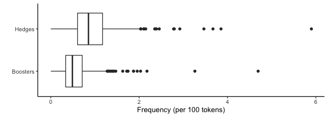
How do these look to you?

Format the data

Now let’s create some data for our regression models. For this, we’ll combine our frequency counts with some metadata: discipline category, speaker status, gender, and paper type. We’ll also move the text_id to row names to exclude that column from further processing.

lr_df <- hb %>%
    mutate(doc_id = str_remove_all(doc_id, ".txt")) %>%
    dplyr::select(doc_id, hedges_norm, boosters_norm) %>%
    left_join(select(micusp_meta, doc_id, discipline_cat, speaker_status,
        student_gender, paper_type), by = "doc_id") %>%
    remove_rownames %>%
    column_to_rownames(var = "doc_id")

For the mulinomial regression, we’re going to want to collapse all of the discipline categories into 3: Science, Humanities, and Social Science.

lr_df$discipline_cat <- str_replace_all(lr_df$discipline_cat, "BIO|CEE|ECO|IOE|MEC|NRE|PHY",
    "SCI")
lr_df$discipline_cat <- str_replace_all(lr_df$discipline_cat, "CLS|ENG|HIS|PHI",
    "HUM")
lr_df$discipline_cat <- str_replace_all(lr_df$discipline_cat, "ECO|EDU|LIN|NUR|POL|PSY|SOC",
    "SOCSCI")

To carry out our regression, we need to convert our character columns to factors. In other words, they need to be treated like categories not strings. We can do them all with one simple line of code.

lr_df <- lr_df %>%
    mutate_if(is.character, as.factor)

Logistic regression model

We’ll start with student gender as our outcome variable and hedges and boosters as our predictors. The family argument specifies logistic regression.

glm_fit1 <- glm(student_gender ~ boosters_norm + hedges_norm, data = lr_df,
    family = "binomial")

And we do something similar for speaker status.

glm_fit2 <- glm(speaker_status ~ boosters_norm + hedges_norm, data = lr_df,
    family = "binomial")

And finally, let’s repeat this process with a subset of our data. We have 3 discipline categories, so let’s subset out only 2.

lr_sub <- lr_df %>%
    filter(discipline_cat == "HUM" | discipline_cat == "SCI")
lr_sub$discipline_cat <- droplevels(lr_sub$discipline_cat)

glm_fit3 <- glm(discipline_cat ~ boosters_norm + hedges_norm, data = lr_sub,
    family = "binomial")

                      ────────────────────────────────────────────────────────────────────────
                                            Model 1           Model 2           Model 3       
                                      ────────────────────────────────────────────────────────
                        (Intercept)            0.50 ***          3.45 ***           6.27 ***  
                                        [0.35, 0.70]      [2.19, 5.43]      [3.66, 10.74]     
                        boosters_norm          1.29              1.92 *             0.03 ***  
                                        [0.86, 1.91]      [1.03, 3.56]       [0.01, 0.06]     
                        hedges_norm            1.07              0.95               1.81 **   
                                        [0.81, 1.43]      [0.66, 1.37]       [1.20, 2.73]     
                                      ────────────────────────────────────────────────────────
                        N                    828               828                462         
                        AIC                 1103.01            775.59             517.76      
                        BIC                 1117.17            789.75             530.16      
                        Pseudo R2              0.00              0.01               0.28      
                      ────────────────────────────────────────────────────────────────────────
                        *** p < 0.001; ** p < 0.01; * p < 0.05.                               

Multinomial regression model

Now let’s try multinomial regression on all 3 of the discipline categories. This isn’t covered in the textbook, but it’s worth looking at even if briefly.

mr_fit <- multinom(discipline_cat ~ boosters_norm + hedges_norm, data = lr_df)

#> # weights:  12 (6 variable)
#> initial  value 909.650975 
#> iter  10 value 814.149632
#> final  value 814.142751 
#> converged

We first see that some output is generated by running the model, even though we are assigning the model to a new R object. This model-running output includes some iteration history and includes the final log-likelihood 814.275451. This value multiplied by two is then seen in the model summary as the Residual Deviance and it can be used in comparisons of nested models.

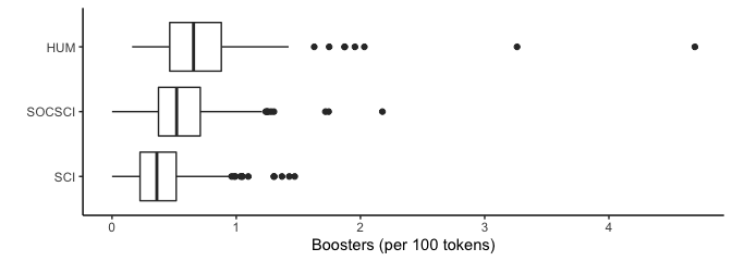
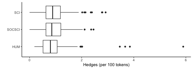
Let’s look at a couple of boxplots to give us some context for these numbers.

ggplot(lr_df, aes(x = reorder(discipline_cat, boosters_norm, FUN = median),
    y = boosters_norm)) + geom_boxplot() + xlab("") + ylab("Boosters (per 100 tokens)") +
    theme_classic() + coord_flip()

ggplot(lr_df, aes(x = reorder(discipline_cat, hedges_norm, FUN = median),
    y = hedges_norm)) + geom_boxplot() + xlab("") + ylab("Hedges (per 100 tokens)") +
    theme_classic() + coord_flip()

Much like logistic regression, th ratio of the probability of choosing one outcome category over the probability of choosing the baseline category is the relative risk or odds. The relative risk is the right-hand side linear equation exponentiated, leading to the fact that the exponentiated regression coefficients are relative risk ratios for a unit change in the predictor variable. We can exponentiate the coefficients from our model to see these odds ratios.

                                  ─────────────────────────────────────────────────
                                                                   Model 1         
                                                          ─────────────────────────
                                    (Intercept)                          1.99 ***  
                                                                  [1.45, 2.53]     
                                    boosters_norm                       -3.92 ***  
                                                                [-4.71, -3.13]     
                                    hedges_norm                          0.59 **   
                                                                  [0.16, 1.01]     
                                                          ─────────────────────────
                                    nobs                               828         
                                    edf                                  6.00      
                                    deviance                          1628.29      
                                    AIC                               1640.29      
                                    nobs.1                             828.00      
                                  ─────────────────────────────────────────────────
                                    *** p < 0.001; ** p < 0.01; * p < 0.05.        

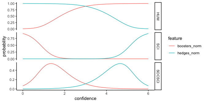
Sometimes a plot can be helpful in interpreting the results. Let’s start by making some dummy data. For this we’ll sequence frequencies of hedges from 0 to 6 percent of a text, and frequencies of boosters on an inverse scale: from 6 to 0 percent of a text. In essence, we creating hypothetical texts that have at one end have low frequencies of hedges and high frequencies of boosters, have balanced frequencies in the middle, and have high frequencies of hedges and low frequencies of boosters.

hb_new <- data.frame(hedges_norm = seq(0, 6, by = 0.1), boosters_norm = seq(6,
    0, by = -0.1))

Next, we create a data frame of discipline probabilities based on our fit.

prob_disc <- cbind(hb_new, predict(mr_fit, newdata = hb_new, type = "probs",
    se = TRUE))

We’ll format a data frame for plotting.

plot_prob <- prob_disc %>%
    pivot_longer(hedges_norm:boosters_norm, names_to = "feature", values_to = "confidence") %>%
    pivot_longer(HUM:SOCSCI, names_to = "variable", values_to = "probability")

Finally, we’ll create a plot the probabilities and color by hedges & boosters.

ggplot(plot_prob, aes(x = confidence, y = probability, color = feature)) +
    geom_line() + theme_classic() + facet_grid(variable ~ ., scales = "free")

Lab 9: Multi-Dimensional Analysis

Multi-Dimensional Analysis (MDA) is a process made up of 4 main steps:

1. Identification of relevant variables

2. Extraction of factors from variables

3. Functional interpretation of factors as dimensions

4. Placement of categories on the dimensions

It is also a specific application of factor analysis. Factor analysis is a method(s) for reducing complexity in linguistic data, which can identify underlying principles of systematic variation (Biber 1988).

library(cmu.textstat)
library(tidyverse)
library(quanteda)
library(nFactors)

Case 1: Biber Tagger

In order to carry out MDA, we would like to have 5 times as many observations than variables. This generally precludes carrying out MDA (or factor analysis) with simple word counts. We need data that has, in some way, been tagged.

For this lab, we will use data prepared using the R package pseudobibeR, which emulates the classification system that Biber has used and reported in much of his research. The package aggregates the lexicogrammatical and functional features widely used for text-type, register, and genre classification tasks.

The scripts are not really taggers. Rather, they use udpipe or spaCy part-of-speech tagging and dependency parsing to summarize patterns. They organize 67 categories.

For this lab, you won’t need to use the package functions. But if you’d like to try it out for any of your projects, you can follow the instructions.

The Brown Corpus

Let’s start with counts from the Brown Corpus. The Brown family of corpora is discussed on pg. 16 of Brezina. You can also find more about it here:

http://icame.uib.no/brown/bcm.html

bc <- read_csv("https://raw.githubusercontent.com/browndw/cmu-textstat-docs/main/docs/_static/labs_files/data-csv/bc_biber.csv",
    show_col_types = FALSE)

bc_meta <- read_csv("https://raw.githubusercontent.com/browndw/cmu-textstat-docs/main/docs/_static/labs_files/data-csv/brown_meta.csv",
    show_col_types = FALSE)

We will join the data with the metadata, in order to calculate dimension scores by register and evaluate them.

Note

The categorical variable must be formatted as a factor. For convenience sake, we’ll move the file names to the row names and put our factor as the first column.

``` r
bc <- bc %>%
    left_join(dplyr::select(bc_meta, doc_id, text_type)) %>%
    mutate(text_type = as.factor(text_type)) %>%
    column_to_rownames("doc_id") %>%
    dplyr::select(text_type, everything())

Correlation matrix

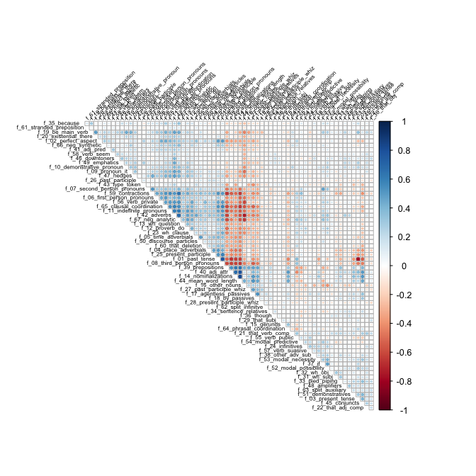
Before calculating our factors, let’s check a correlation matrix. Note that we’re dropping the first (factor) column.

bc_cor <- cor(bc[-1], method = "pearson")

corrplot::corrplot(bc_cor, type = "upper", order = "hclust", tl.col = "black",
    tl.srt = 45, diag = F, tl.cex = 0.5)

Determining number of factors

Typically, the number of factors is chosen after inspecting a scree plot.

screeplot_mda(bc)

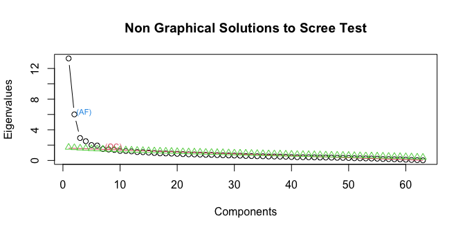
A common method for interpreting a scree plot is to look for the “bend” in the elbow, which would be 3 or 4 factors in this case. We can also look at the results of other kinds of solutions like optimal coordinates, which measures the gradients associated with eigenvalues and their preceding coordinates, and acceleration factor, which determines the coordinate where the slope of the curve changes most abruptly. In this case OC suggests 6 factors and AF 1.

For the purposes of this exercise, we’ll start with 3 factors.

Calculating factor loadings and MDA scores

In factor analysis factors so that they pass through the middle of the relevant variables. For linguistic variable it is conventional to use a promax rotation (see Brezina pgs. 164-167). There is also a nice explanation of rotations here:

https://personal.utdallas.edu/~herve/Abdi-rotations-pretty.pdf

To place our categories along the dimensions, data is standardized by converting to z-scores. For each text, a dimension score is calculated by summing all of the high-positive variables subtracting all of the high-negative variables. Then, the mean is calculated for each category.

For these calculations, we will use the mda_loadings() function.

bc_mda <- mda_loadings(bc, n_factors = 3)

We can access factor loadings and group means through attributes: attr(bc_mda, "loadings")

	Factor1	Factor2	Factor3
f_01_past_tense	-0.15	1.10	0.16
f_02_perfect_aspect	0.05	0.52	0.28
f_03_present_tense	0.60	-1.06	-0.04
f_04_place_adverbials	0.17	0.42	-0.11
f_05_time_adverbials	0.23	0.32	0.06
f_06_first_person_pronouns	0.44	0.15	0.22
f_07_second_person_pronouns	0.66	-0.11	-0.14
f_08_third_person_pronouns	0.19	0.73	0.16
f_09_pronoun_it	0.32	0.11	0.39
f_10_demonstrative_pronoun	0.36	-0.15	0.37
f_11_indefinite_pronouns	0.49	0.30	0.26
f_12_proverb_do	0.54	0.04	0.14
f_13_wh_question	0.39	0.10	0.05
f_14_nominalizations	-0.51	-0.39	0.21
f_15_gerunds	-0.02	-0.16	-0.03
f_16_other_nouns	-0.29	-0.32	-0.77
f_17_agentless_passives	-0.48	-0.21	0.00
f_18_by_passives	-0.45	-0.16	0.02
f_19_be_main_verb	0.46	-0.09	0.41
f_20_existential_there	0.13	0.13	0.30
f_21_that_verb_comp	-0.18	0.08	0.44
f_22_that_adj_comp	0.01	-0.10	0.38
f_23_wh_clause	0.36	0.23	0.22
f_24_infinitives	0.10	0.01	0.24
f_25_present_participle	0.12	0.48	-0.03
f_27_past_participle_whiz	-0.53	0.08	-0.11
f_28_present_participle_whiz	-0.22	0.03	-0.16
f_30_that_obj	0.00	-0.11	0.26
f_31_wh_subj	-0.14	-0.10	0.14
f_32_wh_obj	-0.03	0.04	0.27
f_33_pied_piping	-0.17	-0.17	0.34
f_34_sentence_relatives	-0.21	-0.07	0.08
f_35_because	0.33	-0.13	0.15
f_36_though	-0.20	0.16	0.32
f_37_if	0.53	-0.27	0.12
f_38_other_adv_sub	0.02	-0.06	0.33
f_39_prepositions	-0.68	-0.23	-0.06
f_40_adj_attr	-0.41	-0.47	0.18
f_41_adj_pred	0.14	0.16	0.26
f_42_adverbs	0.57	0.21	0.51
f_43_type_token	0.14	0.12	-0.06
f_44_mean_word_length	-0.65	-0.36	0.04
f_45_conjuncts	-0.20	-0.41	0.37
f_46_downtoners	0.13	-0.03	0.38
f_47_hedges	0.40	0.10	0.24
f_48_amplifiers	0.04	-0.11	0.36
f_49_emphatics	0.41	-0.26	0.26
f_50_discourse_particles	0.41	0.07	0.00
f_51_demonstratives	-0.10	-0.31	0.31
f_52_modal_possibility	0.45	-0.39	0.29
f_53_modal_necessity	0.10	-0.36	0.19
f_54_modal_predictive	0.43	-0.12	-0.09
f_55_verb_public	0.07	0.38	0.09
f_56_verb_private	0.25	0.44	0.44
f_57_verb_suasive	-0.12	0.03	0.03
f_58_verb_seem	-0.02	0.13	0.39
f_59_contractions	0.61	0.25	-0.03
f_60_that_deletion	0.25	0.26	0.03
f_63_split_auxiliary	-0.04	-0.07	0.37
f_64_phrasal_coordination	-0.15	-0.39	-0.02
f_65_clausal_coordination	0.47	0.37	0.28
f_66_neg_synthetic	0.07	0.32	0.35
f_67_neg_analytic	0.57	0.20	0.38

Plotting the results

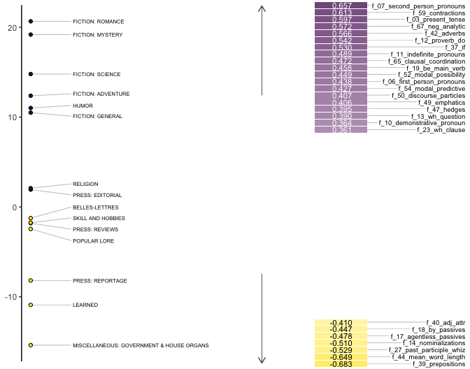
The means are conventionally positioned on a stick plot of the kind Brezina shows on pg. 169.

mda.biber::stickplot_mda(bc_mda, n_factor = 1)

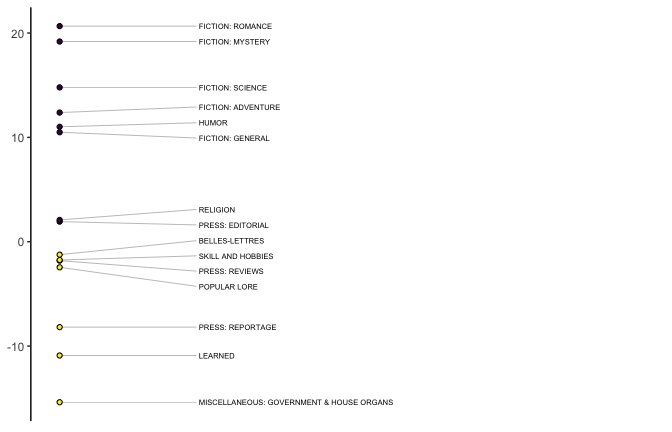
We can also show the same plot with the factor loadings.

mda.biber::heatmap_mda(bc_mda, n_factor = 1)

Evaluating MDA

Typically, MDA is evaluated using ANOVA, reporting the F statistic, degrees of freedom, and R-squared. We can extract that information from a linear model.

f_aov <- aov(Factor1 ~ group, data = bc_mda)
broom::tidy(f_aov)
#> # A tibble: 2 × 6
#>   term         df  sumsq meansq statistic   p.value
#>   <chr>     <dbl>  <dbl>  <dbl>     <dbl>     <dbl>
#> 1 group        14 51553.  3682.      32.1  3.49e-60
#> 2 Residuals   485 55651.   115.      NA   NA

f1_lm <- lm(Factor1 ~ group, data = bc_mda)
names(f1_lm$coefficients) <- names(coef(f1_lm)) %>%
    str_remove("group")
f2_lm <- lm(Factor2 ~ group, data = bc_mda)
names(f2_lm$coefficients) <- names(coef(f2_lm)) %>%
    str_remove("group")
f3_lm <- lm(Factor3 ~ group, data = bc_mda)
names(f3_lm$coefficients) <- names(coef(f3_lm)) %>%
    str_remove("group")

                     ──────────────────────────────────────────────────────────────────────────
                                                       Factor 1      Factor 2      Factor 3    
                                                    ───────────────────────────────────────────
                       (Intercept)                     -1.24         -0.81          1.73 *     
                       FICTION: ADVENTURE              13.62 ***     14.80 ***     -0.81       
                       FICTION: GENERAL                11.73 ***     13.40 ***     -0.23       
                       FICTION: MYSTERY                20.43 ***     14.38 ***      3.10       
                       FICTION: ROMANCE                21.90 ***     14.09 ***      2.93 *     
                       FICTION: SCIENCE                16.03 ***      8.13 **       5.42       
                       HUMOR                           12.25 **       7.28 ***      2.94       
                       LEARNED                         -9.66 ***     -7.75 ***     -0.11       
                       MISCELLANEOUS: GOVERNMENT &    -14.14 ***     -9.57 ***     -9.19 ***   
                       HOUSE ORGANS                                                            
                       POPULAR LORE                    -1.21         -0.58         -2.37       
                       PRESS: EDITORIAL                 3.17         -2.28         -0.87       
                       PRESS: REPORTAGE                -6.94 ***      0.71        -10.37 ***   
                       PRESS: REVIEWS                  -0.57         -2.89         -3.85 *     
                       RELIGION                         3.33         -3.82 *        4.29 *     
                       SKILL AND HOBBIES               -0.51         -5.56 ***     -5.09 ***   
                                                    ───────────────────────────────────────────
                       DF                             485.00        485.00        485.00       
                       R2                               0.48          0.66          0.27       
                       F statistic                     32.09         67.70         13.00       
                     ──────────────────────────────────────────────────────────────────────────
                       *** p < 0.001; ** p < 0.01; * p < 0.05.                                 

Case 2: DocuScope

Unlike the Biber tagger, DocuScope is a dictionary based tagger. It has been developed at CMU by David Kaufer and Suguru Ishizaki since the early 2000s.

Load the dicitonary

DocuScope is a very large dictionary (or lexicon) that organizes tens of millions of words and phrases into rhetorically oriented categories. It has some overlap with a few Biber’s functional categories (like hedges), but is fundamentally different, as it isn’t bases on parts-of-speech.

The ds_dict is a small quanteda dictionary that organizes a reduced set of words of phrases (tens of thousands rather than tens of millions). Here is a sample from 3 of the categories:

ds_dict[1:3]
#> Dictionary object with 3 key entries.
#> - [AcademicTerms]:
#>   - a chapter in, a couple, a declaration of, a detail, a distinction between, a domain, a force, a forced, a form of, a grade, a hint of, a home for, a hub, a kind of, a kind of a, a load, a loaded, a metaphor for, a mix of, a mixture of [ ... and 8,884 more ]
#> - [AcademicWritingMoves]:
#>   - . in this article ,, . in this paper, . this essay, . this paper, . this report, . this work, . to avoid, a better understanding, a common problem, a debate about, a debate over, a first step, a goal of, a great deal of attention, a huge problem, a key to, a major problem, a method of, a notion that, a number of studies [ ... and 1,141 more ]
#> - [Character]:
#>   - ; block, ; bring, ; call, ; center, ; check, ; chill, ; close, ; color, ; control, ; cook, ; cool, ; cover, ; cross, ; cut, ; design, ; discard, ; don, ; down, ; drain, ; e-mail [ ... and 18,754 more ]

Tokenize the corpus

Again, we will use the micusp_mini, and we’ll begin by tokenizing the data. Note that we’re retaining as much of the original data as possible including punctuation. This is because our dictionary includes punctuation marks in it’s entries.

micusp_tokens <- micusp_mini %>%
    corpus() %>%
    tokens(remove_punct = F, remove_numbers = F, remove_symbols = F, what = "word")

Next, we will use the tokens_lookup() function to count and categorize our features.

ds_counts <- micusp_tokens %>%
    tokens_lookup(dictionary = ds_dict, levels = 1, valuetype = "fixed") %>%
    dfm() %>%
    convert(to = "data.frame") %>%
    as_tibble()

Finally, we need to normalize the counts. Because DocuScope is not categorizing ALL of our tokens, we need a total count from the original tokens object.

tot_counts <- quanteda::ntoken(micusp_tokens) %>%
    data.frame(tot_counts = .) %>%
    tibble::rownames_to_column("doc_id") %>%
    dplyr::as_tibble()

ds_counts <- dplyr::full_join(ds_counts, tot_counts, by = "doc_id")

Now we can normalize by the total counts before preparing the data for factor analysis.

ds_counts <- ds_counts %>%
    dplyr::mutate_if(is.numeric, list(~./tot_counts), na.rm = TRUE) %>%
    dplyr::mutate_if(is.numeric, list(~. * 100), na.rm = TRUE) %>%
    dplyr::select(-tot_counts)

ds_counts <- ds_counts %>%
    mutate(text_type = str_extract(doc_id, "^[A-Z]+")) %>%
    mutate(text_type = as.factor(text_type)) %>%
    column_to_rownames("doc_id")

Calculating factor loadings and MDA score

Again, we will use 3 factors.

micusp_mda <- mda_loadings(ds_counts, n_factors = 3)

Evaluating MDA

We can again check to see how explanatory our dimensions are.

f1_lm <- lm(Factor1 ~ group, data = micusp_mda)
names(f1_lm$coefficients) <- names(coef(f1_lm)) %>%
    str_remove("group")
f2_lm <- lm(Factor2 ~ group, data = micusp_mda)
names(f2_lm$coefficients) <- names(coef(f2_lm)) %>%
    str_remove("group")
f3_lm <- lm(Factor3 ~ group, data = micusp_mda)
names(f3_lm$coefficients) <- names(coef(f3_lm)) %>%
    str_remove("group")

                              ─────────────────────────────────────────────────────────
                                               Factor 1      Factor 2      Factor 3    
                                            ───────────────────────────────────────────
                                (Intercept)    -2.81 **       4.44 ***     -0.54       
                                CEE            -4.31 **      -1.25          0.17       
                                CLS             7.71 ***     -7.65 ***     -1.72       
                                ECO             0.40         -3.29          3.50 *     
                                EDU             5.82 ***     -2.86          2.97 *     
                                ENG            10.28 ***     -8.22 ***     -2.17       
                                HIS             4.81 **     -10.06 ***     -3.22 *     
                                IOE            -0.30         -4.06 *        3.40 *     
                                LIN             2.77         -0.53         -0.99       
                                MEC            -4.82 **      -1.33         -0.51       
                                NRE             0.20         -8.46 ***      3.03 *     
                                NUR             3.37 *       -3.37          5.23 ***   
                                PHI             9.49 ***     -1.62         -0.73       
                                PHY            -1.91         -1.06         -1.30       
                                POL             6.00 ***    -13.21 ***      1.47       
                                PSY             3.16 *       -1.35          0.07       
                                SOC             5.15 ***     -7.23 ***     -0.00       
                                            ───────────────────────────────────────────
                                DF            153.00        153.00        153.00       
                                R2              0.65          0.51          0.39       
                                F statistic    17.49          9.77          6.01       
                              ─────────────────────────────────────────────────────────
                                *** p < 0.001; ** p < 0.01; * p < 0.05.                

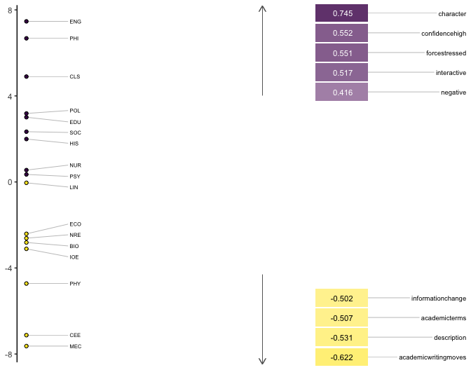
Plotting the results

And we can plot the first factor.

mda.biber::heatmap_mda(micusp_mda, n_factor = 1)

Interpreting the factors as dimensions

The functional interpretation of factors as dimensions (Brezina pgs. 167-168) is probably the most challenging part of MDA. As analysts, we need to make sense out of why features (whether parts-of-speech, rhetorical categories, or other measures) are grouping together and contributing to the patterns of variation evident in products of the analysis.

That interpretation usually involves giving names to the dimensions based on their constituent structures. In Biber’s original study, he called his first, most explanatory dimension Involved vs. Informational Production. At the positive (Involved) end of the dimension are telephone and face-to-face conversations. At the negative (Information) end are official documents and academic prose.

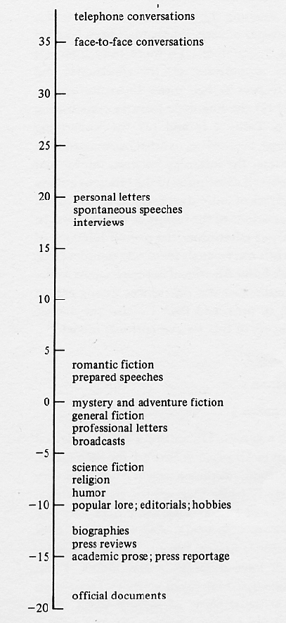
Features with high positive loadings include private verbs (like think), contractions, and first and second person pronouns. Features with high negative loadings include nouns and propositional phrases. Biber concludes that these patterns reflect the communicative purposes of the registers. Ones that are more interactive and affective vs. others that are more instructive and informative.

Factor 1
private verbs	0.96
that deletion	0.91
contractions	0.9
present tense verbs	0.86
2nd person pronouns	0.86
do as pro-verb	0.82
analytic negation	0.78
demonstrative pronouns	0.76
general emphatics	0.74
1st person pronouns	0.74
pronoun it	0.71
be as main verb	0.71
causative subordination	0.66
discourse particles	0.66
indefinite pronouns	0.62
hedges	0.58
amplifiers	0.56
sentence relatives	0.55
wh- questions	0.52
possibility modals	0.5
non-phrasal coordination	0.48
wh- clauses	0.47
final prepositions	0.43
nouns	-0.8
word length	-0.58
prepositions	-0.54
type/ token ratio	-0.54
attributive adjectives	-0.47

In order to understand how certain features are functioning, it is important to see how they are being used, which we can do effienciently with Key Words in Context (KWIC). Here we take “Confidence High” from the positive end of the dimension and “Academic Writing Moves” from the negative using the kwic() function.

ch <- kwic(micusp_tokens, ds_dict["ConfidenceHigh"])

awm <- kwic(micusp_tokens, ds_dict["AcademicWritingMoves"])

docname	from	to	pre	keyword	post	pattern
BIO.G0.02.1	191	191	sympatry ; do these examples	simply	represent another head on the	ConfidenceHigh
BIO.G0.02.1	401	402	speciation in this genus ,	most likely	under sympatric conditions . The	ConfidenceHigh
BIO.G0.02.1	708	708	that this mechanism is not	very	efficient , and depends on	ConfidenceHigh
BIO.G0.02.1	1143	1143	normal host species respond in	predictable	manners : choosing to mate	ConfidenceHigh
BIO.G0.02.1	1425	1426	explored later ; however ,	it is	important to note here that	ConfidenceHigh
BIO.G0.02.1	1718	1718	of finding a mate that	knows	the same song as you	ConfidenceHigh

docname	from	to	pre	keyword	post	pattern
BIO.G0.02.1	258	260	, yet another possible example	has been described	by science , which may	AcademicWritingMoves
BIO.G0.02.1	594	596	, this type of behavior	has been observed	in the indigobirds of Vidua	AcademicWritingMoves
BIO.G0.02.1	913	914	( Lonchura striata ) .	They conducted	a second experiment in 2000	AcademicWritingMoves
BIO.G0.02.1	939	940	1998 study . Their experiment	was designed	principally to test three hypotheses	AcademicWritingMoves
BIO.G0.02.1	1019	1020	, the Bengalese , finch	were used	. In the cross-foster experiments	AcademicWritingMoves
BIO.G0.02.1	1204	1205	sometime before fledging - this	finding is	also consistent with Payne et	AcademicWritingMoves