Set 02

The goal of this first lab set is to introduce:

• How to produce and interpret token frequencies

• How to produce and interpret token distributions

• Some basic principles of token distributions in a corpus

Lab 4: Distributions

Prepare a corpus

Load the needed packages

library(cmu.textstat)
library(tidyverse)
library(quanteda)
library(quanteda.textstats)

Load a corpus

The cmu.textstat package comes with some data sets including a data table with a column of document ids and a column of texts. Such a table is easy to create from text data on your own local drive.

To do so, you would organize plain .txt files into a directory and use the readtext() function from the readtext package.

sc_df <- sample_corpus

To peek at the data, we’ll look at the first 100 characters in the text column of the first row:

Teachers and other school personnel are often counseled to use research findings in making curricula

Make a corpus object.

sc <- corpus(sc_df)

And check the result:

Text	Types	Tokens	Sentences
acad_01	842	2816	95
acad_02	983	2829	88
acad_03	969	2887	126
acad_04	1017	2860	102
acad_05	914	2834	109
acad_06	1007	2813	86

Document variables (Name your files systematically!)

Note the names of the text files encode important meta-data: in this case, the names of text types similar to the Corpus of Contemporary American English.

This is extremely important. When you build your own corpora, yo want to purposefully and systematically name your files and organize your directories. This will save you time and effort later in your analysis.

We are now going to extract the meta-data from the file names and pass them as a variable.

doc_categories <- str_extract(sc_df$doc_id, "^[a-z]+")

Check the result:

acad
blog
fic
mag
news
spok
tvm
web

We will now assign the variable to the corpus. The following command might look backwards, with the function on the left hand side of the <- operator. That is because it’s an accessor function, which lets us add or modify data in an object. You can tell when a function is an accessor function like this because its help file will show that you can use it with <-, for example in ?docvars.

docvars(sc, field = "text_type") <- doc_categories

And check the summary again:

Text	Types	Tokens	Sentences	text_type
acad_01	842	2816	95	acad
acad_02	983	2829	88	acad
acad_03	969	2887	126	acad
acad_04	1017	2860	102	acad
acad_05	914	2834	109	acad
acad_06	1007	2813	86	acad

Tokenize the corpus

We’ll use quanteda to tokenize. And after tokenization, we’ll convert them to lower case. Why do that here? As a next step, we’ll being combining tokens like a and lot into single units. And we’ll be using a list of expressions that isn’t case sensitive.

sc_tokens <- tokens(sc, include_docvars = TRUE, remove_punct = TRUE, remove_numbers = TRUE,
    remove_symbols = TRUE, what = "word")

sc_tokens <- tokens_tolower(sc_tokens)

Multi-word Expressions

An issue that we run into frequently with corpus analysis is what to do with multi-word expressions. For example, consider a common English quantifier: a lot. Typical tokenization rules will split this into two tokens: a and lot. But counting a lot as a single unit might be important depending on our task. We have a way of telling quanteda to account for these tokens.

All that we need is a list of multi-word expressions.

The cmu.textstat comes with an example of an mwe list called multiword_expressions:

winter haven
with a view to
with reference to
with regard to
with relation to
with respect to

The tokens_compound() function looks for token sequences that match our list and combines them using an underscore.

sc_tokens <- tokens_compound(sc_tokens, pattern = phrase(multiword_expressions))

Create a document-feature matrix

With our tokens object we can now create a document-feature-matrix using the dfm() function. As a reminder, a dfm is table with one row per document in the corpus, and one column per unique token in the corpus. Each cell contains a count of how many times a token shows up in that document.

sc_dfm <- dfm(sc_tokens)

Next we’ll create a http://quanteda.io/reference/dfm_weight.html with proportionally weighted counts.

prop_dfm <- dfm_weight(sc_dfm, scheme = "prop")

Token distributions

Distributions of the

Let’s start by selecting frequencies of the most common token in the corpus:

freq_df <- textstat_frequency(sc_dfm) %>%
    data.frame(stringsAsFactors = F)

feature	frequency	rank	docfreq	group
the	50910	1	399	all
and	25222	2	398	all
to	24749	3	397	all
of	22057	4	399	all
a	21605	5	398	all
in	15964	6	399	all
i	12560	7	348	all
that	12529	8	396	all
you	10948	9	341	all
is	9895	10	389	all

From the weighted dfm, we can select any token that we’d like to look at more closely. In this case, we’ll select the most frequent token: the.

After selecting the variable, we will convert the data into a more friendly data structure.

There are easier ways of doing this, but the first bit of the code-chunk allows us to filter by rank and return a character vector that we can pass. This way, we can find a word of any arbitrary rank.

Also note how the rename() function is set up. Let’s say our token is the. The dfm_select() function would result with a column named the that we’d want to rename RF. So our typical syntax would be: rename(RF = the). In the chunk below, however, our column name is the variable word. To pass that variable to rename, we use !!name(word).

word <- freq_df %>%
    filter(rank == 1) %>%
    dplyr::select(feature) %>%
    as.character()

word_df <- dfm_select(prop_dfm, word, valuetype = "fixed")  # select the token

word_df <- word_df %>%
    convert(to = "data.frame") %>%
    cbind(docvars(word_df)) %>%
    rename(RF = !!as.name(word)) %>%
    mutate(RF = RF * 1e+06)

With that data it is a simple matter to generate basic summary statistics using the group_by() function:

summary_table <- word_df %>%
    group_by(text_type) %>%
    summarize(MEAN = mean(RF), SD = sd(RF), N = n())

text_type	MEAN	SD	N
acad	68619.15	18327.65	50
blog	51268.52	13391.02	50
fic	54201.50	14254.59	50
mag	57086.29	14007.56	50
news	50482.34	18485.42	50
spok	42812.15	9787.92	50
tvm	32532.85	11981.88	50
web	60600.51	21646.94	50

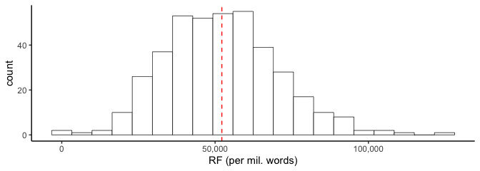
And we can inspect a histogram of the frequencies. To set the width of our bins we’ll use the Freedman-Diaconis rule. The bin-width is set to:

\[h = 2 x \frac{IQR(x)}{n^{1/3} }\]

Note

Other popular methods for calculating optimal bin width include “Scott’s rule”.

So the number of bins is (max-min)/h, where n is the number of observations, max is the maximum value and min is the minimum value.

bin_width <- function(x) {
    2 * IQR(x)/length(x)^(1/3)
}

Now we can plot a histogram. We’re also adding a dashed line showing the mean. Note we’re also going to use the scales package to remove scientific notation from our tick labels.

ggplot(word_df, aes(RF)) + geom_histogram(binwidth = bin_width(word_df$RF),
    colour = "black", fill = "white", size = 0.25) + geom_vline(aes(xintercept = mean(RF)),
    color = "red", linetype = "dashed", size = 0.5) + theme_classic() +
    scale_x_continuous(labels = scales::comma) + xlab("RF (per mil. words)")

Distributions of the and of

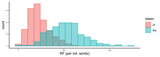
Now let’s try plotting histograms of two tokens on the same plot. First we’re going to use regular expressions (^the$|^of$) to select the columns. The carat or hat ^ looks for the start of line. Without it, we would also get words like blather. The dollar symbol $ looks for the end of a line. The straight line | means “or”. Think about how useful this flexibility can be. You could, for example, extract all words that end in -ion.

# Note 'regex' rather than 'fixed'
word_df <- dfm_select(prop_dfm, "^the$|^of$", valuetype = "regex")

# Now we'll convert our selection and normalize to 10000 words.
word_df <- word_df %>%
    convert(to = "data.frame") %>%
    mutate(the = the * 10000) %>%
    mutate(of = of * 10000)

# Use 'pivot_longer' to go from a wide format to a long one
word_df <- word_df %>%
    pivot_longer(!doc_id, names_to = "token", values_to = "RF") %>%
    mutate(token = factor(token))

Now let’s make a new histogram. Here we assign the values of color and fill to the token column. We also make the columns a little transparent using the alpha setting.

ggplot(word_df, aes(x = RF, color = token, fill = token)) + geom_histogram(binwidth = bin_width(word_df$RF),
    alpha = 0.5, position = "identity") + theme_classic() + xlab("RF (per mil. words)") +
    theme(axis.text = element_text(size = 5))

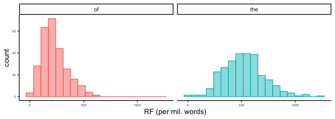
If we don’t want overlapping histograms, we can use facet_wrap() to split the plots.

ggplot(word_df, aes(x = RF, color = token, fill = token)) + geom_histogram(binwidth = bin_width(word_df$RF),
    alpha = 0.5, position = "identity") + theme_classic() + theme(axis.text = element_text(size = 5)) +
    theme(legend.position = "none") + xlab("RF (per mil. words)") + facet_wrap(~token)

Dispersion

We can also calculate dispersion, and there are a variety of measures at our disposal. Our toolkit has several functions for producing these calculations.

For example, we can find the dispersion of any specific token:

the <- dispersions_token(sc_dfm, "the") %>%
    unlist()

Absolute frequency	50910.000
Per_10.5	5239.482
Relative entropy of all sizes of the corpus parts	1.000
Range	399.000
Maxmin	292.000
Standard deviation	45.937
Variation coefficient	0.361
Chi-square	6310.987
Juilland et al.’s D (based on equally-sized corpus parts)	0.982
Juilland et al.’s D (not requiring equally-sized corpus parts)	0.982
Carroll’s D2	0.989
Rosengren’s S (based on equally-sized corpus parts)	0.963
Rosengren’s S (not requiring equally-sized corpus parts)	0.966
Lyne’s D3 (not requiring equally-sized corpus parts)	0.968
Distributional consistency DC	0.963
Inverse document frequency IDF	0.004
Engvall’s measure	50782.725
Juilland et al.’s U (based on equally-sized corpus parts)	49990.109
Juilland et al.’s U (not requiring equally-sized corpus parts)	50000.041
Carroll’s Um (based on equally sized corpus parts)	50331.945
Rosengren’s Adjusted Frequency (based on equally sized corpus parts)	49022.075
Rosengren’s Adjusted Frequency (not requiring equally sized corpus parts)	49167.056
Kromer’s Ur	2135.467
Deviation of proportions DP	0.139
Deviation of proportions DP (normalized)	0.139

And let’s try another token to compare:

data <- dispersions_token(sc_dfm, "data") %>%
    unlist()

	the	data
Deviation of proportions DP	0.139	0.846

Deviation of proportions is a useful measure as it accounts for the relative sizes of the corpus parts (see Brezina pg. 52). Thus, it works well when a corpus is made up of texts with unequal lengths. It is calculated as follows (Greis 2008, p. 415):

1. Determine the sizes s_1−n of each of the n corpus parts, which are normalized against the overall corpus size and correspond to expected percentages which take differently-sized corpus parts into consideration.

2. Determine the frequencies v_1−n with which a occurs in the n corpus parts, which are normalized against the overall number of occurrences of a and correspond to observed percentages.

3. Compute all n pairwise absolute differences of observed and expected percentages, sum them up, and divide the result by two. The result is DP, which can theoretically range from approximately 0 to 1, where values close to 0 indicate that a is distributed across the n corpus parts as one would expect given the sizes of the n corpus parts. By contrast, values close to 1 indicate that a is distributed across the n corpus parts exactly the opposite way one would expect given the sizes of the n corpus parts.

Dispersions for all tokens

We can also calculate selected dispersion measures for all tokens using dispersions_all():

d <- dispersions_all(sc_dfm)

Token	AF	Per_10.5	Carrolls_D2	Rosengrens_S	Lynes_D3	DC	Juillands_D	DP	DP_norm
the	50910	5239.482	0.989	0.966	0.968	0.963	0.982	0.139	0.139
and	25222	2595.761	0.990	0.969	0.973	0.967	0.984	0.124	0.124
to	24749	2547.082	0.993	0.980	0.983	0.976	0.987	0.090	0.090
of	22057	2270.030	0.978	0.933	0.935	0.932	0.974	0.199	0.200
a	21605	2223.512	0.992	0.976	0.978	0.973	0.986	0.109	0.110
in	15964	1642.960	0.988	0.962	0.963	0.960	0.981	0.146	0.146

Generating a frequency table

Alternatively, frequency_table() returns only Deviation of Proportions and Average Reduced Frequency.

Note that ARF requires a tokens object and takes a couple of minutes to calculate.

ft <- frequency_table(sc_tokens)

	Token	AF	Per_10.5	ARF	DP
1	the	50910	5239.482	31893.812	0.139
2	and	25222	2595.761	15905.994	0.124
3	to	24749	2547.082	15464.035	0.090
5	of	22057	2270.030	13086.919	0.199
4	a	21605	2223.512	13233.050	0.109
6	in	15964	1642.960	9766.973	0.146

Note

In addition to a dfm of normalized frequencies (like we did above), we can create a term frequency-inverse document frequency (tf-idf) matrix using the dfm_tfidf() function.

A tf-idf is a popular weighting scheme (particularly in text classificaation tasks) that attempts to account for both token frequency and dispersion. A tf–idf value increases proportionally according to the number of times a token appears in the document and is offset by the number of documents in the corpus that contain the token.

Zipf’s Law

Let’s plot rank (along the x-axis) against frequency (along the y-axis) for the 100 most frequent tokens in the sample corpus.

ggplot(freq_df %>%
    filter(rank < 101), aes(x = rank, y = frequency)) + geom_point(shape = 1,
    alpha = 0.5) + theme_classic() + ylab("Absolute frequency") + xlab("Rank")

The relationship you’re seeing between the rank of a token and it’s frequency holds true for almost any corpus and is referred to as Zipf’s Law (see Brezina pg. 44).

Lab 5: Collocations

This is a short lab that introduces the concept of:

• collocations,

• how to calculate word association measures like pointwise mutual information, and

• how to plot collocational networks.

This lab will also cover the process of reading in a corpus from a directory of text files.

Load the needed packages

library(cmu.textstat)
library(tidyverse)
library(quanteda)
library(quanteda.textstats)
library(ggraph)

Prepare the data

First, we’ll pre-process our text, create a corpus and tokenize the data:

sc_tokens <- sample_corpus %>%
  mutate(text = preprocess_text(text)) %>%
  corpus() %>%
  tokens(what="fastestword", remove_numbers=TRUE)

Collocates by mutual information (MI)

The collocates_by_MI() function produces collocation measures (by pointwise mutual information) for a specified token in a quanteda tokens object. In addition to a token, a span or window (as given by a number of words to the left and right of the node word) is required. The default is 5 to the left and 5 to the right.

The formula for calculating MI is as follows:

\[log_{2} \frac{O_{11}}{E_{11}}\]

Where O₁₁ and E₁₁ are the observed (i.e., node + collocate) and expected frequencies of the node word within a given window. The expected frequency is given by:

\[E_{11} = \frac{R_{1} \times C_{1}}{N}\]

• N is the number of words in the corpus

• R₁ is the frequency of the node in the whole corpus

• C₁ is the frequency of the collocate in the whole corpus

We’ll start by making a table of tokens that collocate with the token money.

money_collocations <- collocates_by_MI(sc_tokens, "money")

Check the result:

token	col_freq	total_freq	MI_1
10:29	1	1	11.08
38th	1	1	11.08
allocations	1	1	11.08
americanizing	1	1	11.08
anthedon	1	1	11.08
assignats	1	1	11.08

Now, let’s make a similar table for collocates of time.

time_collocations <- collocates_by_MI(sc_tokens, "time")

token	col_freq	total_freq	MI_1
decleat	2	1	10.135
poignantly	2	1	10.135
16a	1	1	9.135
17a	1	1	9.135
21h	1	1	9.135
aba	1	1	9.135

As is clear from the above table, MI is sensitive to rare/infrequent words (see Brezina pg. 74). Because of that sensitivity, it commmon to make thresholds for both token frequency (absolute frequency) and MI score (usually at some value ≥ 3).

For our purposes, we’ll filter for AF ≥ 5 and MI ≥ 5.

tc <- time_collocations %>% filter(col_freq >= 5 & MI_1 >= 5)
mc <- money_collocations %>% filter(col_freq >= 5 & MI_1 >= 5)

Check the result:

token	col_freq	total_freq	MI_1
warner	6	8	8.720
cessation	5	7	8.650
irradiation	5	7	8.650
lag	5	7	8.650
wasting	7	11	8.483
frame	7	16	7.943

token	col_freq	total_freq	MI_1
owe	5	21	9.010
raise	10	79	8.099
extra	6	64	7.665
spend	10	111	7.608
insurance	5	64	7.402
spent	9	122	7.320

Create a tbl_graph object for plotting

A tbl_graph is a data structure for tidyverse (ggplot2) network plotting.

For this, we’ll use the col_network() function.

net <- col_network(tc, mc)

Plot network

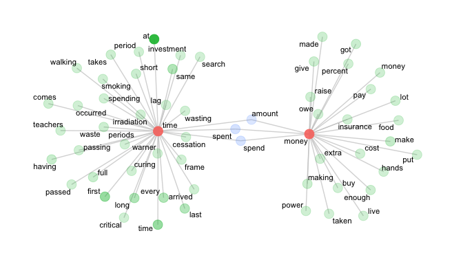
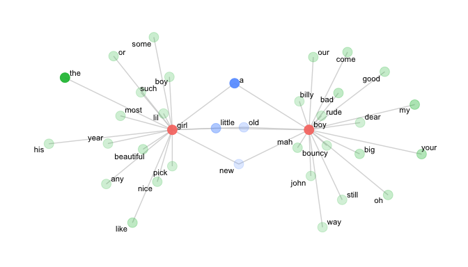
The network plot shows the tokens that distinctly collocate with either time or money, as well as those that intersect. The distance from the central tokens (time and money) is governed by the MI score and the transparency (or alpha) is governed by the token frequency.

The aesthetic details of the plot can be manipulated in the various ggraph options.

ggraph(net, weight = link_weight, layout = "stress") + 
  geom_edge_link(color = "gray80", alpha = .75) + 
  geom_node_point(aes(alpha = node_weight, size = 3, color = n_intersects)) +
  geom_node_text(aes(label = label), repel = T, size = 3) +
  scale_alpha(range = c(0.2, 0.9)) +
  theme_graph() +
  theme(legend.position="none")

Reading in local files

Create a vector of file paths

First, go to Canvas and dowload the screenplay_corpus (in the Data folder under Files). Unzip the corpus and note/copy the path to the folder.

Next, we’ll create a vector of the file paths. Remember to replace your/path with the place-holder path in the list.files() function.

files_list <- list.files("your/path", full.names = T, pattern = "*.txt")

Read in files using readtext

Next, we’ll read in the files using readtext. And for the purposes of efficiency, we’ll sample out 50 files from the paths vector.

set.seed(1234)

sp <- sample(files_list, 50) %>%
  readtext::readtext()

Extract the dialogue

These particular files are formatted using some simple markup. So we’ll use the from_play() function to extract the dialogue.

sp <- from_play(sp, extract = "dialogue")

Tokenize

sp <-   sp %>%
  mutate(text = preprocess_text(text)) %>%
  corpus() %>%
  tokens(what="fastestword", remove_numbers=TRUE)

Calculate MI

Now we’ll calculate collocations for the tokens boy and girl, and filter. Note that we’re only looking for tokens 3 words to the left of the node word.

b <- collocates_by_MI(sp, "boy", left = 3, right = 0)
b <- b %>% filter(col_freq >= 3 & MI_1 >= 3)

g  <- collocates_by_MI(sp, "girl", left = 3, right = 0)
g <- g %>% filter(col_freq >= 3 & MI_1 >= 3)

Plot the network

net <- col_network(b, g)

ggraph(net, weight = link_weight, layout = "stress") + 
  geom_edge_link(color = "gray80", alpha = .75) + 
  geom_node_point(aes(alpha = node_weight, size = 3, color = n_intersects)) +
  geom_node_text(aes(label = label), repel = T, size = 3) +
  scale_alpha(range = c(0.2, 0.9)) +
  theme_graph() +
  theme(legend.position="none")

See other examples hereand here.

Lab 6: Keyness

For this lab, we’ll be following many of the same procedures that we’ve done previously:

• attaching metadata to a corpus using docvars()

• tokenizing using tokens()

• handling multiword expressions using tokens_compound()

• creating a document-feature matrix using dfm()

For today’s lab we’ll begin some hypothesis testing using news functions from quanteda.extras:

• keyness_table()

• keyness_pairs()

• key_keys()

We’ll also look at quanteda’s function:

• textstat_keyness()

What is keyness?

Keyness is a generic term for various tests that compare observed vs. expected frequencies.

The most commonly used (though not the only option) is called log-likelihood in corpus linguistics, but you will see it else where called a G-test goodness-of-fit.

The calculation is based on a 2 x 2 contingency table. It is similar to a chi-square test, but performs better when corpora are unequally sized.

Expected frequencies are based on the relative size of each corpus (in total number of words N_i) and the total number of observed frequencies:

\[E_i = \sum_i O_i \times \frac{N_i}{\sum_i N_i}\]

And log-likelihood is calculted according the formula:

\[LL = 2 \times \sum_i O_i \ln \frac{O_i}{E_i}\]

A good explanation of its implementation in linguistics can be found here: http://ucrel.lancs.ac.uk/llwizard.html

In addition to log-likelihood, the textstat_keyness() function in quanteda has other optional measures.

See here: https://quanteda.io/reference/textstat_keyness.html

Prepare a corpus

We’ll begin, just as we did in the distributions lab.

Load the needed packages

library(cmu.textstat)
library(tidyverse)
library(quanteda)
library(quanteda.textstats)

Pre-process the data & create a corpus

sc <- sample_corpus %>%
  mutate(text = preprocess_text(text)) %>%
  corpus()

Extract meta-data from file names

We’ll extract some meta-data by (1) selecting the doc_id column, (2) extracting the initial letter string before the underscore, and (3) renaming the vector text_type.

doc_categories <- sample_corpus %>%
  dplyr::select(doc_id) %>%
  mutate(doc_id = str_extract(doc_id, "^[a-z]+")) %>%
  rename(text_type = doc_id)

Assign the meta-data to the corpus

The accessor function docvars() lets us add or modify data in an object. We’re going to use it to assign text_type as a variable. Note that doc_categories could include more than one column and the assignment process would be the same.

docvars(sc) <- doc_categories

And check the result:

Text	Types	Tokens	Sentences	text_type
acad_01	772	2534	1	acad
acad_02	933	2544	1	acad
acad_03	889	2525	1	acad
acad_04	941	2541	1	acad
acad_05	857	2504	1	acad
acad_06	962	2575	1	acad

Note

We could assign the new column (text_type on the right) any number of categorical variables to our corpus, which could be used for analysis downstream.

Create a dfm

sc_dfm <- sc %>%
  tokens(what="fastestword", remove_numbers=TRUE) %>%
  tokens_compound(pattern = phrase(multiword_expressions)) %>%
  dfm()

A corpus composition table

It is conventional to report out the composition of the corpus or corpora you are using for your study. Here will will sum our tokens by text-type and similarly count the number of texts in each grouping.

We will also use janitor to append a row of totals at the bottom of the table.

corpus_comp <- ntoken(sc_dfm) %>% 
  data.frame(Tokens = .) %>%
  rownames_to_column("Text_Type") %>%
  mutate(Text_Type = str_extract(Text_Type, "^[a-z]+")) %>%
  group_by(Text_Type) %>%
  summarize(Texts = n(),
    Tokens = sum(Tokens)) %>%
  mutate(Text_Type = c("Academic", "Blog", "Fiction", "Magazine", "News", "Spoken", "Television/Movies", "Web")) %>%
  rename("Text-Type" = Text_Type) %>%
  janitor::adorn_totals()

Text-Type	Texts	Tokens
Academic	50	121442
Blog	50	125492
Fiction	50	128644
Magazine	50	126631
News	50	119029
Spoken	50	127156
Television/Movies	50	128191
Web	50	124302
Total	400	1000887

Keyness in quanteda

Now that we have a dfm we perform keyness calculations. First, let’s carry out calculations using textstat_keyness().

When we use it with textstat_keyness we are indicating that we want the papers with discipline_cat equal to “acad” to be our target corpus. The everything else (i.e., "acad” == FALSE) will be the reference corpus.

The specific method we’re using is log-likelihood, which is designated by lr. Thus keyness will show the tokens that are more frequent in papers written for the academic text-type vs. those written for other text-types.

acad_kw <- textstat_keyness(sc_dfm, docvars(sc_dfm, "text_type") == "acad", measure = "lr")

Note

The slightly awkward syntax of the second argument docvars(sc_dfm, “text_type”) == “acad” simply produces a logical vector. You could store it and pass the vector the function, as well.

feature	G2	p	n_target	n_reference
of	1703.9045	0	4848	17258
the	777.8819	0	8273	42712
social	456.0039	0	208	133
studies	391.0565	0	155	71
study	318.9471	0	158	119
in	316.6583	0	2715	13341
perfectionism	301.8410	0	74	1
by	297.3255	0	790	2707
practice	267.9016	0	117	68
science	259.3673	0	118	75
students	244.5197	0	146	150
patients	240.5276	0	90	35
results	238.7283	0	105	62
changes	237.4097	0	121	96
research	237.2037	0	151	170
et_al	225.7370	0	66	9
learning	224.0288	0	89	41
model	201.4563	0	90	55
education	197.9501	0	107	94
methylation	197.1762	0	49	1

Creating sub-corpora

If we want to compare one text-type (as our target corpus) to another (as our reference corpus), we can easily subset the data.

sub_dfm <- dfm_subset(sc_dfm, text_type == "acad" | text_type == "fic")

When we do this, the resulting data will still include all the tokens in the sample corpus, including those that do not appear in either the academic or fiction text-type. To deal with this, we will trim the dfm

sub_dfm <- dfm_trim(sub_dfm, min_termfreq = 1)

We’ll dow the same for fiction.

fic_kw <- textstat_keyness(sub_dfm, docvars(sub_dfm, "text_type") == "fic", measure = "lr")

feature	G2	p	n_target	n_reference
i	2350.2083	0	2428	143
she	1861.4841	0	1763	70
he	1699.1024	0	1978	170
her	1453.0085	0	1559	104
you	1361.1128	0	1286	50
n’t	929.2936	0	914	43
his	805.0630	0	1155	157
my	732.2578	0	758	44
me	591.5002	0	557	21
him	541.5136	0	548	29
said	415.0374	0	474	38
d	390.2396	0	427	30
it	352.8352	0	1449	567
was	342.6948	0	1535	630
had	313.5124	0	837	243
up	307.6199	0	429	55
like	271.4322	0	433	70
back	264.8461	0	305	25
eyes	221.6091	0	181	2
know	218.6785	0	253	21

Note that if we switch our target and reference corpora (academic as target, fiction as reference), the tail of the keyness table contains the negative values of the original (fiction as target, academic and reference), which you may have already gathered given the formula above.

acad_kw <- textstat_keyness(sub_dfm, docvars(sub_dfm, "text_type") == "acad", measure = "lr")

feature	G2	p	n_target	n_reference
of	1260.3272	0	4848	2153
the	266.0260	0	8273	6768
social	248.2684	0	208	7
are	222.0430	0	707	276
studies	213.2714	0	155	1
by	209.9241	0	790	342
in	189.3192	0	2715	1922
students	179.4487	0	146	4
research	175.2807	0	151	6
is	173.0845	0	1241	720
study	170.2493	0	158	9
political	162.7745	0	134	4
changes	157.0893	0	121	2
these	151.9318	0	267	61
results	141.7558	0	105	1
science	140.6435	0	118	4
also	138.4218	0	224	46
education	137.3372	0	107	2
based	132.3798	0	112	4
such_as	130.2988	0	102	2

Effect size

While quanteda produces one important piece of information (the amount of evidence we have for an effect), it neglects another (the magnitude of the effect). Whenever we report on significance it is critical to report effect size. Some common effect size measures include:

• %DIFF - see Gabrielatos and Marchi (2012)

  • Costas has also provided an FAQ with more details

• Bayes Factor (BIC) - see Wilson (2013)

  • You can interpret the approximate Bayes Factor as degrees of evidence against the null hypothesis as follows:

    • 0-2: not worth more than a bare mention

    • 2-6: positive evidence against H₀

    • 6-10: strong evidence against H₀

    • 10: very strong evidence against H₀

  • For negative scores, the scale is read as “in favor of” instead of “against”.

• Effect Size for Log Likelihood (ELL) - see Johnston et al (2006)

  • ELL varies between 0 and 1 (inclusive). Johnston et al. say “interpretation is straightforward as the proportion of the maximum departure between the observed and expected proportions”.

• Relative Risk

• Odds Ratio

• Log Ratio - see Andrew Hardie’s CASS blog for how to interpret this

  • Note that if either word has zero frequency then a small adjustment is automatically applied (0.5 observed frequency which is then normalized) to avoid division by zero errors.

Log Ratio (LR)

You are welcome to use any of these effect size measures. Our cmu.textstat package comes with a function for calculating Hardie’s Log Ratio, which is easy and intuitive.

The keyness_table() function

We’ll start by creating 2 dfms–a target and a reference:

acad_dfm <- dfm_subset(sc_dfm, text_type == "acad") %>% dfm_trim(min_termfreq = 1)
fic_dfm <- dfm_subset(sc_dfm, text_type == "fic") %>% dfm_trim(min_termfreq = 1)

Then we will use the keyness_table() function.

acad_kw <- keyness_table(acad_dfm, fic_dfm)

And check the result:

Token	LL	LR	PV	AF_Tar	AF_Ref	Per_10.5_Tar	Per_10.5_Ref	DP_Tar	DP_Ref
of	1225.7730	1.2541581	0	4848	2153	3992.02912	1673.610895	0.0924456	0.1511810
the	250.0277	0.3727977	0	8273	6768	6812.30546	5261.030441	0.1055235	0.0984965
social	248.0959	4.9762015	0	208	7	171.27518	5.441373	0.6466724	0.8803364
are	221.1949	1.4401587	0	707	276	582.17091	214.545568	0.2064176	0.3007237
studies	213.1703	7.3592411	0	155	1	127.63294	0.777339	0.6724121	0.9800068
by	208.9950	1.2909730	0	790	342	650.51630	265.849942	0.1653887	0.2219184
in	185.8180	0.5814606	0	2715	1922	2235.63512	1494.045583	0.1123519	0.0905818
students	179.3624	5.2729413	0	146	4	120.22200	3.109356	0.7959013	0.9397640
research	175.1907	4.7365590	0	151	6	124.33919	4.664034	0.6265416	0.9002208
is	171.7388	0.8685510	0	1241	720	1021.88699	559.684089	0.2251045	0.3636254
study	170.1541	4.2169725	0	158	9	130.10326	6.996051	0.5088941	0.8399537
political	162.7021	5.1492059	0	134	4	110.34074	3.109356	0.7070091	0.9199030
changes	157.0286	6.0019800	0	121	2	99.63604	1.554678	0.6880038	0.9602469
these	151.7452	2.2130753	0	267	61	219.85804	47.417680	0.2622432	0.4710608
results	141.7094	6.7973622	0	105	1	86.46103	0.777339	0.5622868	0.9804344
science	140.5877	4.9657598	0	118	4	97.16573	3.109356	0.8023869	0.9395153
also	138.2830	2.3669097	0	224	46	184.45019	35.757595	0.2738380	0.5192314
education	137.2899	5.8245837	0	107	2	88.10790	1.554678	0.7864189	0.9600370
based	132.3297	4.8904716	0	112	4	92.22510	3.109356	0.4528605	0.9211234
such_as	130.2558	5.7555421	0	102	2	83.99071	1.554678	0.3484990	0.9603868

The columns are as follows:

1. LL: the keyness value or log-likelihood, also know as a G2 or goodness-of-fit test.

2. LR: the effect size, which here is the log ratio

3. PV: the p-value associated with the log-likelihood

4. AF_Tar: the absolute frequency in the target corpus

5. AF_Ref: the absolute frequency in the reference corpus

6. Per_10.x_Tar: the relative frequency in the target corpus (automatically calibrated to a normalizing factor, where here is per 100,000 tokens)

7. Per_10.x_Ref: the relative frequency in the reference corpus (automatically calibrated to a normalizing factor, where here is per 100,000 tokens)

8. DP_Tar: the deviation of proportions (a dispersion measure) in the target corpus

9. DP_Ref: the deviation of proportions in the reference corpus

Keyness pairs

There is also a function for quickly generating pair-wise keyness comparisions among multiple sub-corpora. To demonstrate, create a third dfm, this time containing news articles.

news_dfm <- dfm_subset(sc_dfm, text_type == "news") %>% dfm_trim(min_termfreq = 1)

To produce a data.frame comparing more than two sup-corpora, use the keyness_pairs() function:

kp <- keyness_pairs(news_dfm, acad_dfm, fic_dfm)

Check the result:

Token	A_v_B_LL	A_v_B_LR	A_v_B_PV	A_v_C_LL	A_v_C_LR	A_v_C_PV	B_v_C_LL	B_v_C_LR	B_v_C_PV
he	492.0071	2.3234670	0	-394.5566793	-1.1338521	0.0000000	-1686.795822	-3.4573191	0.0000000
said	455.3403	3.6879174	0	1.9426817	0.1302184	0.1633777	-414.325296	-3.5576990	0.0000000
i	430.9713	2.3569230	0	-853.6051892	-1.6456416	0.0000000	-2330.444833	-4.0025647	0.0000000
n’t	333.0647	3.2283984	0	-173.1956844	-1.0982705	0.0000000	-926.435351	-4.3266689	0.0000000
you	327.5135	3.0610552	0	-410.9814035	-1.5406468	0.0000000	-1355.342948	-4.6017020	0.0000000
mr	236.5815	5.0950435	0	75.2537234	1.6133756	0.0000000	-60.919384	-3.4816679	0.0000000
park	226.4408	8.3598712	0	139.4716944	3.1950604	0.0000000	-25.260727	-5.1648108	0.0000005
she	212.5637	2.3631957	0	-919.2114232	-2.2082213	0.0000000	-1850.638989	-4.5714170	0.0000000
p.m	209.5632	8.2481229	0	199.7074846	6.3312396	0.0000000	-2.659024	-1.9168833	0.1029639
ob	198.3115	8.1685057	0	206.6332910	8.2516224	0.0000000	0.000000	0.0831167	1.0000000
his	172.3293	1.6200300	0	-244.1842340	-1.1759097	0.0000000	-801.353402	-2.7959397	0.0000000
says	148.6361	3.2936576	0	0.0024484	0.0075405	0.9605356	-151.532656	-3.2861171	0.0000000
s	148.4443	0.8094017	0	0.3913315	0.0358527	0.5316003	-138.681336	-0.7735491	0.0000000
cinemark	137.8335	7.6436642	0	143.6174647	7.7267809	0.0000000	0.000000	0.0831167	1.0000000
kick	129.3948	7.5525163	0	106.8096424	4.6356330	0.0000000	-5.318048	-2.9168833	0.0211056
chang	116.7366	7.4039938	0	121.6351997	7.4871105	0.0000000	0.000000	0.0831167	1.0000000
a.m	113.9236	7.3688043	0	87.1022425	4.1299930	0.0000000	-6.647560	-3.2388114	0.0099292
hall	110.0188	6.4383453	0	37.7853395	1.8210223	0.0000000	-27.457875	-4.6173230	0.0000002
gur	106.8913	7.2768819	0	111.3768094	7.3599986	0.0000000	0.000000	0.0831167	1.0000000
run	103.7965	3.2592520	0	69.0483759	2.1848274	0.0000000	-5.365009	-1.0744246	0.0205447

Key key words

The concept of “key key words” was introduced by Mike Smith for the WordSmith concordancer. The process compares each text in the target corpus to the reference corpus. Log-likelihood is calculated for each comparison. Then a mean is calculated for keyness and effect size. In addition, a range is provided for the number of texts in which keyness reaches significance for a given threshold. (The default is p < 0.05.) That range is returned as a percentage.

In this way, key key words accounts for the dispersion of key words by indicating whether a keyness value is driven by a relatively high frequency in a few target texts or many.

kk <- key_keys(acad_dfm, fic_dfm)

Again, we can look at the first few rows of the table:

token	key_range	key_mean	key_sd	effect_mean
of	98	59.20	36.40	1.21
social	38	25.00	70.11	3.41
studies	44	22.56	67.90	5.93
students	16	19.64	70.17	3.56
the	64	17.80	26.72	0.31
research	34	17.57	63.50	3.48

Key key words when comparing the academic text-type to the fiction text-type.